Masters Project

Analysis of the U.S. Natural Gas Pipeline System With Respect to Leaks.

Natalie A. Sullo

A Special Project

Submitted in Partial Fulfillment of the

Requirements for the Degree of

Master of Arts in Statistics

Department of Mathematics

Central Connecticut State University

New Britain, Connecticut

December 2013

Department of Mathematical Sciences

Keywords: Natural gas pipelines, generalized linear model, negative binomial regression.

ABSTRACT

The prevalence of leaks within the natural gas pipeline system of the United States is analyzed based on variables consisting of: location, material, and diameter. Causes of the leaks are attributed to corrosion, natural forces, third party damage, material defects, construction defects, excavation, and variable other causes that are investigated. A negative binomial regression was used to model the data of the natural gas pipeline leaks and to predict the number of leaks in the existing natural gas pipelines. This model helped determine which pipelines are more susceptible to specific leaks in order to prevent each type of leak and reduce the risk of accidents. Transmission and distribution companies and their pipelines were examined separately and the data is represented individually.

It is found that steel cathodically protected bare is the most common material found in transmission natural gas pipelines and this material predicts fewer leaks then its steel unprotected and bare counterparts. Cast wrought iron predicts the least number of leaks compared to the other materials for transmission onshore pipelines.

Pipeline materials in distribution pipelines differ from those of transmission pipelines. The most common materials are cathodically protected coated steel and plastic. Plastic shows to be a preferred material when looking at leaks from corrosion of pipelines, however plastic pipelines are limited to those with less pressure, making plastic more common in distribution pipelines where the pipes are carrying less gas and generally under less pressure.

This study shows that there is not one material that outperforms the others in all causes of leaks, and some materials work better in specific environments than in others. It is necessary to consider the location of the pipeline and the nature of the gas being carried in order to accurately select the best material for that situation.

INTRODUCTION

Natural gas is a colorless and odorless gas found under the earth’s surface. Natural gas companies have taken various trajectories in their methods for obtaining, transporting, and delivering this resource to their consumers. Given the large demand for natural gas, many companies find themselves at a crossroads to determine what would be the best method for updating the pipeline system that is both costs efficient for the companies and also safe for its consumers.

Given the financial necessities, many companies have not updated their systems resulting in unnecessary leaks that can lead to dangerous situations to the public. It is important to look at the overall functioning of the pipeline system in order to propose a possible change to better it. By looking at why leaks are occurring, it will be easier and more cost efficient to repair or replace the system.

1.1 HISTORY AND BACKGROUND OF NATURAL GAS

Natural gas was first identified in the United States by French explorers in 1626 as they witnessed Native Americans igniting the fuel around Lake Erie as it seeped through the Earth’s crust. The significance of natural gas as an energy source was nonexistent at the time; it was not until the past few decades that people were able to establish methods for containing and using the gas (“NaturalGas.org”).

Historically, natural gas, which is commonly found near oil, was deemed useless and burnt off. Today, it has become an important energy source as it can be found in various sectors ranging from residential to industrial.

William Hart, known as the “father of natural gas”, created the first natural gas well, in Fredonia, New York in 1821. The well was 27 feet deep, allowing Hart to extract the gas and contain it. From this he created the first natural gas company named Fredonia Gas Light Company (“History Zone”). His endeavor established the significance of natural gas. Today natural gas is one of the most widely used resources’ accounting for 24 percent of the total energy consumed in the United States (“NaturalGas.org”).

Colonel Edwin Drake marked the beginning of the transportation pipeline system in the United States in 1859. He created a 69-foot well that collected gas and transported it by means of a pipeline, which was 2 inches in diameter and 5.5 miles long in Titusville, Pennsylvania. This was the start of the first natural gas pipeline system in the United States (“NaturalGas.org”).

In 1872 the Rochester Natural Gas Light Company was formed. This company transported natural gas 25 miles to the city of Rochester, New York. The pipeline system was made of hollowed-out Canadian white pine logs, which soon rotted and ceased to function (Nersesian, 2007). To improve the natural gas transportation system, pipelines started being made from different materials such as cast and wrought-iron. These too had many problems since “Cast and wrought-iron pipelines were plagued by breaks and leaking connections held together by screws” (Nersesian, 2007). These pipes were improved with larger diameters, and leak-proof rubber rings in the pipe joints.

In the 1880’s the use of electric lights became widespread, taking away business from natural gas companies. Given the introduction of electric lighting, gas companies switched their focus from lights to cooking and heating. This required natural gas companies to create pipelines to enter homes and buildings directly (Nersesian, 2007). These kinds of pipelines are called distribution and service pipelines and will be looked at later in our analysis.

Also in the 1880’s, George Westinghouse, who was one of the largest natural gas distributors in Pittsburgh and an advocate for safety, created a pipe around his main gas pipelines to contain leaks. He also used pressure regulators to reduce gas pressure in homes, and made safety cutoff valves, which detected low pressure to stop the gas in case of leaks (Nersesian, 2007). These safety mechanisms put in place were so efficient that some of these techniques are still used today.

New technological advances were developed during the interwar period, throughout and after World War II, between the 1920’s to the 1960’s. These pipelines were different than any previous pipelines built because they were made with better metal materials and incorporated welding and pipe rolling. During this time thousands of miles of durable pipelines were constructed. Natural gas was used to heat homes, heat water, and operate ovens. It was also used commercially in manufacturing, generating electricity, and even transportation (“NaturalGas.org”).

In 1935 there were only four natural gas companies with Standard Oil of New Jersey controlling 60 percent of all the pipelines. The Public Holding Act of 1935 was passed to make locally managed pipeline companies, breaking up the monopoly (Nersesian, 2007, p. 235). A few years later the Natural Gas Act of 1938 made for regulation of interstate pipelines requiring companies to document operations and financial matters.

Natural gas has proven itself to be a favorable source of energy for environmental and efficiency reasons. It is the cleanest burning fossil fuel and emits only water and carbon dioxide when burned (Nersesian, 2007, p. 225). It is more favorable than oil because it requires little processing and does not require pumping, which can be costly and less efficient. Natural gas is more readily available as its reserves have been estimated to be double that of oil (Nersesian, 2007, p. 225). Using the pipeline system, natural gas is provided to its customers, which allows for a constant flow that is more convenient than other energy sources in comparison to oil or propane, which requires periodic deliveries to establishments and residences. Luckily, these benefits of natural gas outweigh the difficulties in transporting it making it a very desirable energy source.

Containing and transporting natural gas, since it is a gas, has proved to be very difficult. The majority of large natural gas deposits are found in remote areas far away from the highly populated destinations that consume it. Nations have developed ways to transport this gas differently. Large deposits found in the island of Trinidad, far from consumers, have been converted into a liquid form and transported by ship to the rest of the world making it a globally traded product. In other parts of the world complex pipeline systems have been built to transport the gas. This is the most common way of exploiting and transporting this natural resource. In Siberia, Russia, there is a transcontinental pipeline system that moves gas over far distances to Europe. There is even a pipeline system under the Mediterranean Sea! The transportation of the natural resource has changed over the years and continues to improve. This method is arduous as there are many difficulties in maintaining the integrity of the many miles of pipelines. Leaking natural gas is very dangerous especially in confined areas where it could asphyxiate people, trigger fires or cause an explosion. This is why great emphasis is placed on maintaining safe and effective transportation methods (Nersesian, 2007, p. 225).

1.2 TODAY’S UNITED STATES NATURAL GAS PIPELINE SYSTEM

Natural gas in the United States is transported by a large pipeline system. Gas is extracted from the earth and brought through pipelines called flowlines to storage units. The gas is then picked up by gathering pipelines and transported to processing or holding facilities, where the gas is processed. Large pipelines called transmission lines transport the gas many miles to local distribution companies. Compressor stations are positioned along the transmission pipeline to ensure adequate pressure. These compressor stations are constantly regulated to ensure efficiency and safety. The gas is then passed off from the transmission company to a distribution company through a gate station. At these stations the pressure in the pipelines is reduced, an odor is added to the gas, and the amount of gas that is being passed through is measured. The gas then leaves the gate station through main pipelines operated by the distribution company. Service pipelines branch off from these main pipelines bringing the gas to individual establishments, which go through a meter before being delivered to the customer.

This paper examines leak data recorded by individual companies on their natural gas pipelines. The data used contains both transmission data and distribution data. The former contains data on gathering pipelines, and transmission pipelines. Both transmission and gathering pipelines are found and recorded as onshore and offshore. This difference in location separates these two types of pipelines into four separate categories; transmission onshore, transmission offshore, gathering onshore, and gathering offshore. It is important to look at gathering and transmission pipelines separately because gathering pipelines transport un-processed gas, which has a different composition that increases the rate of corrosion and can have other effects on the integrity of the pipelines. Onshore and offshore pipelines should be considered separately also because of the different environments in which they exist. Comparing these different locations and gas forms could be of interest with relation to leaks. The lengths of these pipelines are measured in miles.

The distribution data file used contains information on both main and service pipelines. The former are measured in miles and the latter are measured by frequency. In general service pipelines are very short (and should be looked at as a “driveway” for gas). Because there is not one main unit of measurement and there is variation in some of the variables (service pipelines are smaller in diameter then main pipelines) they cannot be combined.

The U.S. system is comprised of over 320,000 miles of transmission and gathering pipelines, and 2,066,000 miles of main and service pipelines. The Pipeline and Hazardous Materials Safety Administration (PHMSA), under the department of transportation, regulates this natural gas pipeline system in the United States. An image of this process provided by the PHMSA can be seen in Figure 1.

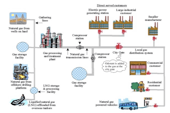
Figure 1. Natural gas pipeline system progression of transportation.

The pipelines that will be investigated within this analysis are from both transmission companies and distribution companies. For transmission companies, both gathering and transmission pipelines will be considered. For distribution companies both main and service pipelines will be considered.

Figure 2 shows a map of the 2009 natural gas transmission pipeline network from the U.S. Energy Information Administration, (EIA). Interstate pipelines are in red and intrastate pipelines are in blue. Most intrastate pipelines are located near gas queries/reservoirs and deliver gas to distribution companies where the gas usually never leaves the state. Transmission pipelines generally travel long distances over state lines to bring the natural gas to distribution companies. Main distribution pipelines can also travel through state lines if the distribution company operates over multiple states. The presence of these intrastate pipelines can be seen off the coast in the Gulf of Mexico where the pipelines can be brought directly to distribution companies within state. There are large deposits, or queries, of natural gas in west Texas, Louisiana, Arkansas, Pennsylvania, and southern Quebec (Hallett & Wright, 2011). These gas queries are evident from the concentration of pipelines in Figure 2. Natural gas is taken from these areas and distributed via the pipeline system to the rest of the country.

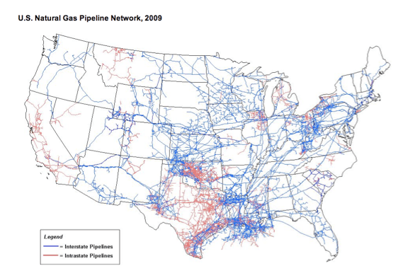
Figure 2. Map of the 2009 natural gas pipeline network of transmission companies from the EIA (www.eia.gov).

1.3 NATURAL GAS PIPELINE LEAKS

To ensure the safety of the public and to reserve the assets of the company, government regulations enforce detection and repair of leaks in the pipelines which are consistently inspected, surveyed, and patrolled to identify and prevent any hazardous situations by fixing leaks at their early stages. Some past leaks that led to the improvement of the natural gas system are discussed below.

In 1906 a major earthquake hit San Francisco, California, which caused gas mains to rupture and started over 30 fires. These fires accounted for most of the damage from the natural disaster. For this reason in some buildings and homes in California “Seismic gas shutoff devices” have been installed, which automatically turn off gas when there is an earthquake of 5.4+ magnitude or greater (“Seismic Gas shut off valves-installation”).

In 1937 in New London, Texas, a natural gas explosion blew up an elementary school killing nearly 300 students and teachers inside (Nersesian, 2007, p. 235). The leak was blamed on a faulty gas line connection. After this explosion it was mandated that an odorant be added to natural gas to aid in the detection of leaks (New London Texas School Explosion).

Pipeline leaks are not just a thing of the past. On September 9^th, 2010 a pipeline in San Bruno, California exploded killing eight people and damaged over 100 homes. A $70 million settlement with Pacific Gas and Electric Company (PG&E), was reached (“San Bruno Announces $70M Blast Settlement with PG&E,” 2012). This pipeline explosion was documented as being due to a paperwork error. After this explosion PG&E was ordered to survey all of its pipelines for possible leaks. They found 46 leaks on high-pressured transmission pipelines like the one that exploded (Worth, 2011).

According to the Pipeline and Hazardous Materials Safety Administration, PHMSA, incidents from natural gas transmission pipelines from 1992-2011, total $1,535,484,409 in property damage, killing 45 people and injuring 216. Those leaks from gathering pipelines total in $356,786,949 worth of property damage with 0 deaths and 12 injuries. Fifty-five percent of these incidents are caused by corrosion, 87% of which being internal corrosion. Distribution pipeline incidents from 1992-2011 totaled $941,868,543 worth of property damage, with 295 deaths and 1,160 injuries. Thirty-six percent of these incidents were due to third party excavation damage, not by an operator/contractor. Additional breakdowns of these incidents by cause are displayed in the pie charts in Figure 3, which are provided from the PHMSA website. This data, which is analyzed separately by pipeline type, gives insight into how these different types of pipelines will differ in their types of leaks within our analysis.

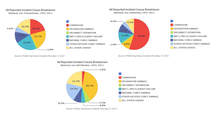Figure 3. Pie chart breakdowns of natural gas leaks on transmission, gathering, and distribution pipelines from the PHMSA.dot.gov/.

BACKGROUND ON DATA

The data used in this paper was provided by the U.S. Department of Transportation under the PHMSA. The data is presently available on the PHMSA website, http://www.phmsa.dot.gov, the exact URL is given in the reference section of this document (PHMSA). This data is obtained from annual, required forms submitted by companies that supply and own natural gas pipelines. A sample of this form is given in Appendix A, which was used by transmission companies between the years 2001 to 2009. Forms from previous years used a similar structure providing slightly different data. This documentation process for submitting information is similar for the distribution companies. The data files are available on the website in Excel format for each individual year from 1990-2010 for distribution and transmission companies separately, so there are 21 files for each type of pipeline. This means there are 21 separate data files for transmission company data and 21 for distribution company data. Data files were merged together using Microsoft Access creating two large data sets, one for transmission data and one for distribution data. It was noted that some of the variables were not the same when merging together these files. The difference between variables and the data preparation taken is discussed in Sections 2.1-2.3. All of the variables used in the analysis are listed in Appendix B.

2.1 DATA VARIABLES

Descriptive variables that appear in both transmission and distribution data sets are year, company name, street, city, state, state of operation, and zip code.

The state of operation variable describes which state the company is operating in. This is usually the same but can be different from the state variable that tells us where the company is based. Onshore transmission companies that transport gas over many states have hubs between states and report pipeline data separately by state even though it could be one continuous pipeline. Distribution companies, which are investor-owned, can also operate across several states. When looking at the data by state, it is assumed that the company is recording the data for that state/region alone. Companies that do operate over more than one state will often operate under different names depending on the state. “For example CenterPoint Energy refers to themselves as Arkla, Entex and Minnegasco depending on which state their operations are in but National Grid may refer to themselves simply as National Grid in NY, RI and MA. This usually happens when a large company (i.e. National Grid) buys smaller distribution companies (i.e. Brooklyn Union, Boston Gas, Rhode Island Gas) and wants to brand them all the same regardless of location” (P. Pierson, Personal communication, April 20, 2012). Some companies that do not record different states separately had more than one state in state of operation variable. Some state of operation variables were missing and the method by which this missing state information was replaced will be discussed in more detail in the data cleansing sections.

The variables region of state, division of state, group of state and Temperature of state were created by using the state of operation variable. The information from the U.S. Census Bureau was used to categorize the states into regions and divisions. Alaska and Hawaii, which are not part of the continental United States, are removed from Division 9 where they are found and put into their own category titled either Region 5 or Division 10. These variables are categorized as follows:

Region 1(Northeast):

Division 1 (New England): CT, ME, MA, NH, RI, and VT

Division 2 (Middle Atlantic): NJ, NY, and PA

Region 2 (Midwest):

Division 3 (East North Central): IN, IL, MI, OH, and WI

Division 4 (West North Central): IA, KS, MO, MN, NE, ND, and SD

Region 3 (South):

Division 5 (South Atlantic): DE, DC, FL, GA, MD, NC, SC, VA, and WV

Division 6 (East South Central): AL, KY, MS, and TN

Division 7 (West South Central): AR, LA, OK, and TX

Region 4 (West):

Division 8 (Mountain): AZ, CO, ID, NM, MT, UT, NV, and WY

Division 9 (Pacific): CA, OR, and WA

Region 5:

Division 10: AK, HI

Region 6:

Division 11: Puerto Rico

States are grouped together based on location and miles of pipelines in each state. These groups outlined below were created using patterns seen in the maps created later in this document.

Group 1: CT, ME, MA, NH, RI, VT

Group 2: NJ, NY, PA

Group 3: IN, IL, MI, OH, WI

Group 4: IA, MO, MN, NE, ND, SD

Group 5: DE, DC, MD, NC, SC, VA, WV, KY, TN

Group 6: KS, AR, OK, MS

Group 7: FL, GA, AL

Group 8: AZ, CO, ID, NM, MT, UT, NV, WY

Group 9: OR, WA

Group 10: LA

Group 11: TX

Group 12: CA

Group 13: AK, HI

Group 14: Puerto Rico

States were also divided into two groups to form Temperature of state; those considered cold weather states with four seasons formed the seasonal region and warm weather states formed the temperate region. This was done to compare temperature conditions for pipelines. The separation of these states was determined by states below the Mason-Dixon Line in the northeast and the average high and low temperatures throughout the United States. The states falling within the two regions are listed below.

Group 1 = Seasonal region = Cold = AK, CO, CT, DE, IA, ID, IL, IN, KS, MA, ME, MI, MN, MO, MS, MT, ND, NE, NH, NJ, NY, OH, OR, PA, RI, SD, UT, VT, WA, WI, and WY.

Group 2 = Temperate region = AL, AR, AZ, CA, DC, FL, GA, HI, KY, LA, MD, MS, NC, NM, NV, OK, SC, TN, TX, VA, WV, Gulf of Mexico, Pacific, and PR.

Miles of pipeline by material tells the number of miles that a company has for each material listed. Each is a continuous numeric variable. Materials that are seen in the transmission data are steel cathodically protected bare, steel cathodically protected coated, steel unprotected bare, steel unprotected coated, cast/wrought iron, plastic, other, and total. Materials seen in distribution data are steel unprotected bare, steel unprotected coated, steel cathodically protected bare, steel cathodically protected coated, plastic all types, plastic PVC, plastic PE, plastic ABS, cast/wrought iron, ductile iron, copper, other_1, other_2, and total miles. Formerly it was believed that cast and wrought iron pipelines (due to its resistance to corrosion) were the best option. However with advances in technology, new materials have become more popular. These cast and wrought iron pipes have more recently been replaced with newer pipelines due to their old age and deterioration. The material of the pipeline also depends on type of pipeline, type of gas, location, local terrain, and pressurization requirements. Two of the most popular pipeline compositions are described by the American Gas Association in the article titled Natural Gas Delivery System are seen below:

“Steel Pipe

Steel is the material used in natural gas transmission systems pipes – these pipes are large in diameter and cover more than a quarter-million miles of our nation. Transmission system pipe is made of 1/4-inch to 1/2-inch thick steel, and has special coatings and “cathodic” protection — an electric current that controls corrosion on the metal surface through electro-chemistry. Some distribution main pipe is also steel, although plastic has become the material of choice for pipe installed in the last 30 years.

Plastic Pipe

During the past 30 years, plastic pipe has predominated in gas utility distribution systems operating at less than 100 pounds of pressure. In 2003, plastic pipe accounted for one-half million miles of distribution main. Plastic pipe is flexible, corrosion-resistant, easy to transport and costs less to install. Plastic pipe also can often be inserted into existing lines or through soil without traditional trenching along its entire route”. (“Natural Gas Delivery System Materials”)

The number of miles of pipeline installed throughout a specific time period is available in the data via variables with the time frame indicated in the name. Two examples of these variables are Transmission – Onshore – Installed – Pre 1940 and Miles of Main Installed – 1940-1949. These variables are categorized in time frames when pipes were installed. These range from unknown, pre-1940, 1940-1949, 1950-1959, 1960-1969, 1970-1979, 1980-1989, 1990-1999, 2000-2009, 2010-2019, and total. These variables of miles installed for each time period are only present after 2003. The problem with these is that some companies report this number differently. These should be recorded as a total new miles of pipelines installed no matter if it is replacing old pipelines or not, however some companies report this number as total net pipelines. “For instance, if they are taking out 12 miles of old steel and replacing it with 12 miles of plastic in one area and just removing 2 miles of old steel in another area, what they really should be reporting is 12 miles of pipe installed. However, what they sometimes report is -2 or (2) miles of pipe installed which isn’t the intent of the question” (P. Pierson, Personal communication, April 20, 2012). Because of this these variables need to be used with caution. Even those with a positive number could be reporting net miles of pipeline without distinguishing between the two. These variables of miles of pipeline within each time frame are recorded for all types of pipeline including gathering, transmission, main, and distribution pipelines.

Both transmission and distribution data sets contain the variable AGA Member which stands for American Gas Association Member. This variable is recorded for years 2002 and later and given a “Y” for yes, the company was a member for that year, and “N” for no, if the company was not a member for that year.

2.2 TRANSMISSION DATA

Transmission data contains gathering and transmission pipelines, both split up into onshore and offshore lines. Gathering pipelines collect or gather the gas from flow lines, the source of the gas, and bring it to processing facilities. These gathering pipelines carry raw gas, or sour-gas, that contains “corrosive content that can affect pipeline integrity within a few years” (Sunshine). At these facilities the gas is processed and then sent long distances to distribution facilities, often times across state lines to where it is taken up by local companies. This is where the gas is handed over to distribution companies and the data for further transportation is seen in the following section on distribution data. Transmission pipelines are generally larger in diameter and transport gas at a higher pressure then other pipelines.

The variables that contain the information on number of leaks are recorded for each company. These exist for multiple causes of leaks. The method in which these variables are recorded changes after 2000. Cause of leaks from 1990-2000 consisted of leaks from corrosion, material defects, outside forces, and other. Causes of leaks from 2001 to 2009 consist of leaks from corrosion, excavation, equipment and operations, material defects, natural forces, other outside forces, and other. In order to create variables that contains valid data from years 1990 to 2009 some variables from the later years are added together. Material defects and equipment and operations are added together to form a Material defects total. Leaks from natural forces, excavation, and other outside forces seen in the data from 2001 to 2009 were added together to form outside forces total where this data completed the outside forces variable given from 1990-2000. This process was done to create uniform variables across all the data. The variables recording leak data used throughout the paper for transmission pipelines are leaks from corrosion, material defects, outside forces, other, and total. These are recorded for transmission onshore pipelines, transmission offshore pipelines, gathering onshore pipelines, and gathering offshore pipelines. These variables are named given the format Leaks – Corrosion – Transmission – Onshore.

Leaks on federal land for onshore and offshore pipelines are also recorded for both gathering and transmission pipelines. Numbers of leaks occurring on an outer continental shelf (OCS) are recorded for transmission and gathering pipes. All of these leaks should be for offshore pipelines since the definition given by the federal government states that the outer continental shelf usually begins 3-9 nautical miles from shore and extends around 200 nautical miles (“The Outer Continental Shelf”).

Onshore gathering and onshore transmission pipelines are separated into four classes. These variables (ex. Gathering- onshore- class 1) give the miles of pipelines that occur in this class. The classes distinguish how populated the area around the pipeline is. Class 1 indicates 10 or less buildings, Class 2 has 10-49 buildings, Class 3 is a mile with more than 49 buildings, and Class 4 is any mile with a four or more story building. The class of the pipeline is used to determine the pipe pressure and wall thickness requirements. These variables are only recorded for years 2001, and 2004 through 2009.

2.3 DISTRIBUTION DATA

Distribution data contains both main and service pipelines recorded separately. The former carry large amounts of gas, and the latter branch from main pipelines to deliver gas to individual homes or buildings. Main and service pipelines can be seen as similar to roads and driveways. Some variables specific to the distribution data set are discussed below.

Pipeline leaks are categorized under one of the following: corrosion, outside force, third party damage, material defect, and other. All of these variables give the number of recorded leaks by cause. Leaks – Corrosion – Mains and Leaks – Corrosion – Services refer to those leaks caused by wear and tear over time, oxidation, etc. Leaks from outside forces can include natural disasters such as hurricanes and earthquakes. Third party damage refers to human damage by vandalism, excavation etc. Material defects occur when the equipment, material or welding is to blame for the leak. This could be the manufacturers fault if a pipeline wall is not thick enough and the gas leaks out.

The variable Percent of Unaccounted for Gas measures amount of gas lost in the pipeline. Natural gas can be measured by volume in cubic feet while under normal temperature and pressure, or in the case of distribution and transmission companies, thousands of cubic feet.

3. RESEARCH QUESTIONS

In this analysis we will be investigating leaks in natural gas pipelines using aforementioned variables to determine the most efficient and safest methods for natural gas pipeline transportation. The variables that we feel are most relevant for establishing a pipeline that would be least prone to leaks are the materials that are used, the diameter of the pipeline, and the location in which they are placed. Spatial correlations will be investigated to determine the differences between the pipeline location by state, region, or group, and onshore versus offshore locations. Temporal analysis will be used to look at the pipeline system over time within the 22 years in which the data spans. The differences between types of pipelines used to transport the gas at different stages of its delivery will also be investigated. Determining which characteristics would make for the most and least effective pipelines would help in the prevention of future leaks.

3.1 RELATIONSHIP OF STUDY TO RELATED RESEARCH

Previous professional literature pertaining to our topic has been reviewed. Natural gas pipeline studies have been conducted but not with regards to types of leaks within such a large data set such as the PHMSA data set used in this study. Some articles of interest pertaining to our research are discussed below.

The study Use of Composite Pipe Materials in the Transportation of Natural Gas by Patrick Laney evaluates the effectiveness of composite materials for transporting natural gas. The purpose of this research is to determine effective materials for transporting the gas, but these do not appear in the data that we will be investigating. This article shows that research is performed in contained environments with the intention on improving materials of pipelines.

There is an abundance of published papers on the analysis of the method in which leaks are detected. However, each of these does not relate directly to the causes of the leaks themselves but only analyzes and discusses how effective each method of detection is. These articles give insight into the different detection methods used for different types of leaks which range from relying on patrons to notify the company about leaks, to physically walking pipeline routes to check for leaks. This article was insightful as to how the leaks in our data set might have been detected. Once pipelines most susceptible to certain leaks are identified, these detection methods could be put in place (Wan, Yu, Wu, Feng, & Yu, 2011).

Regression analysis has shown to be successful in previous pipeline analysis. In the article (Rui, Metz, Reynolds, Chen, & Zhou, 2011) found in the Oil & Gas Journal, regression models are built to predict the price of pipeline projects. In the United States 412 onshore pipelines were used to build the regression models discussed in this paper. This analysis breaks up the geography of the United States into six regions. The variables included in this model are length of pipeline, region, and cross-sectional areas (used instead of diameter which allowed for more accurate evaluation). These were used to build multiple nonlinear regression models for costs from material, labor, miscellaneous, right-of-way, and total cost. The analysis shows a large cost difference between regions. The Southeast region (which includes Florida, Mississippi, Alabama, Georgia, South Carolina, North Carolina, Tennessee, and Kentucky) shows the highest overall costs, contributed by the highest construction and miscellaneous costs. The Northeast has the highest cost of labor, which in my analysis might make for lack of willingness to replace old pipelines. The Midwest and Southwest regions have the highest cost of obtaining the legal right to lay pipelines, which is called right-of-way costs. Also discussed in this article is how the concentration of pipelines affects economic outcomes in the analysis. “Economy of scale tends to arise when firms or projects in the same industry are close together”. Since 40% of the US pipelines studied are located in the Northeast, mainly in Pennsylvania, this concentration reduces the cost. The cost differences between regions can also be attributed to material and right-of-way costs and geographic factors like terrain and population density, weather conditions, soil properties, cost of living, and distance from supplies. This information is interesting to keep in mind when interpreting our analysis (Rui, Metz, Reynolds, Chen, & Zhou, 2011).

In the article (“EXTERNAL CORROSION,” 2009) cathodically protected steel is compared to non-cathodically protected steel. This study concludes “cased pipe segments could be less safe than uncased segments, although this result is not conclusive.” Pipes with cathodic protection are connected to an external power source to provide a current, making the pipeline a cathode of an electrochemical cell, which protects the pipeline from corrosion. This article states that shorts on these cathodically protected pipelines can increase the chance of corrosion. The data used was from the US Office of Pipeline Safety Record Database and only contained two companies that distinguished between whether these pipelines had casting shorts or not. The PHMSA data used in my analysis does not distinguish whether the cathodically protected pipelines were shorted or not, however we can look carefully at cathodically versus non-cathodically protected pipelines to see if this makes a significant difference in preventing leaks (“EXTERNAL CORROSION,” 2009).

In 1999 a study was done on the Department of Transportation Statistics that found over the 16 years prior to 1999 there was no significant change in pipeline accidents, most of these being from human error. In order to try to decrease this number, there should be more knowledgeable persons managing the pipelines, enforcing safety programs, and marking pipeline routes (Hovey & Farmer, 1999).

Another article in the Oil & Gas Journal titled “Risk-based model aids selection of pipeline inspection, maintenance strategies” looks at a small case study analyzing six segments of pipelines, 25-260 kilometers long, over a variety of terrain and conditions to predict causes of different types of leaks. The study finds that pipelines in slushy areas are more susceptible to external corrosion, and those submerged in water are more susceptible to internal corrosion. More frequent leaks due to third party activity are seen in areas where coal is abundant, and also where pipelines cross through rivers. Populated areas are more likely to have leaks from vandalism. Pipelines in rocky areas have more leaks from construction and material defects, which also lead to more leaks from natural forces. Offshore pipelines are more susceptible to leaks from human error and natural causes (“Risk-based,” 2001). These associations are very relevant to our analysis. This study only looks at six different pipelines but gives a basis of things to investigate and think about when analyzing many different pipelines.

This special project extends this existing research by the PHMSA data set with more advanced statistical models. Our research is the first we know of to use this specific dataset to discover such associations with regard to leaks.

3.2 SIGNIFICANCE OF RESEARCH

PHMSA could use this study to reform natural gas pipeline regulations to ensure fewer leaks and increase the overall safety of the system. Gas companies would be interested in this study to create better pipelines that are less likely to leak which reduces costs. This paper looks at the different attributes of the pipelines that make for the best and most efficient system. Identifying which pipelines are more likely to have leaks can allow for companies to concentrate their pipeline repair efforts on these variables. Early detection of leaks will lessen economic loss and environmental pollution. Knowing certain pipelines are susceptible to specific kinds of leaks, a prevention plan tailored to this can be put into effect.

3.3 METHODOLOGY

Data sets for each year from 1990 to 2010 were examined individually to make sure they contained the identical names for the same variables. All 22 data sets were reformatted and merged together by variable name with Microsoft Access. The IBM SPSS Modeler program was also used to merge together data in the 2010 transmission file due to the different formats used. The complete data sets for both distribution and transmission pipeline data were then imported into the IBM SPSS Statistics software where the analyses were performed separately for transmission data and distribution data.

3.4 PROPOSED ANALYSIS

Using information from previous pipeline studies and from exploratory data analysis of the data, we design analyses around what seems to be strong associations of interest in the natural gas pipeline industry. Relationships of the location of pipelines, material, and diameter will be investigated in further detail, which will determine predictors for natural gas pipeline leaks.

To account for the miles of pipelines in each company, leak rates are calculated. These rates are defined as “number of leaks/miles of pipelines,” which adjusts for the miles of pipeline by company. These rates are also calculated for different causes or types of leaks, for example, the number of leaks caused by corrosion per mile of pipeline. The difficulty with this calculated variable is that it is out of total miles of pipeline with all materials, and does not distinguish between which material or diameter of pipe that the leaks occurs on.

To investigate geographical location, data is analyzed by state, region, and group as previously outlined. Graphical map displays are created to visually interpret the differences between leaks in various locations. In previous studies done on natural gas pipelines it has shown that these geographical differences have a big effect on the outcome of the study. It is important to investigate spatial location to determine the effect that this has on the data. These different areas will be looked at individually to determine which grouping of states, if any, has a better potential for predicting the number of leaks.

The simplest count model is based on the Poisson distribution, so we start with a Poisson, or log linear regression model, which is a form of a generalized linear model (GLM), was investigated to be used to model pipeline leaks. This regression is used to model count variables, which would be the number of leaks based on predictors such as material, diameter, and location. The response variable Y is the number of leaks and would contain a number of categories for all types of leaks (corrosion, outside force, third party damage, etc.). This regression was performed separately on different kinds of leaks to compare the different predictors with respect to the types of leaks. A Poisson model was built for each type of leak.

ln(µ) = α + β₁X₁ + β₂X₂ + β₃X₃ + … + β_nX_n,

where µ = E(Y), so that the expected value of Y is E(Y)=µ=e^α * e^β1X1 * e^β2X2 * e^β3X3*…* e^βnXn. To find the predicted probability of the number of leaks we can use the equation:

P(Y_i=y)= (e^-μi * μ_i^y) / y!.

This regression can also be used for rate values that are discussed above where Y=count and Y/t=rate.

In order to perform a Poisson regression model on the data set it is necessary to test if the mean of the data being predicted equals the variance of the data. This is one of the assumptions of the Poisson regression model and if the variance is greater than the mean a negative binomial regression model is needed, which is given below.

ln(µ)= α + β₁X₁ + β₂X₂ + β₃X₃ + … + β_nX_n.

Where the mean =µ = p*r / (1-p), and p is the probability of occurring. To account for varying counts in different records, an additional term is added into the equation using ln(offset variable), called an offset, and creates the equation

ln(µ)= ln(N_n) + α + β₁X₁ + β₂X₂ + β₃X₃ + … + β_nX_n.

The likelihoods of the negative binomial are different from the Poisson and require a different method for fitting the model with a probability mass function of:

P(Y=y) = * (1-p)^r* p^y.

The difference in the miles of leaks per company was accounted for by using exposure, which is an adjustment for the total miles to form rates. To account for the varying total miles of pipelines in each company the log of the exposure variable will be included in the model.

The different types of pipelines were analyzed separately to compare the difference between distribution main and service pipelines, transmission, and gathering pipelines and also between onshore and offshore pipelines. The most significant may vary drastically due to location, material, size, and the different forms of the natural gas being transported (untreated gas versus treated gas could affect the pipeline’s ability to withstand leaks differently).

TRANSMISSION PIPELINE ANALYSIS

Transmission pipeline data include both onshore and offshore transmission and onshore and offshore gathering pipelines. By looking at the data by year it can be seen that the format for collecting the data has significantly changed between the years 2000 and 2001. Another big change is obvious in 2010 when the data for the year was reported over eight separate Excel spreadsheets instead of one. Each of these separate sheets had the variables report number, company, and state of operation in each. Company and state of operation were both used in IBM SPSS Modeler to merge together the separate sheets so that the companies could have all variables in one row in the same spreadsheet. Report number was used initially to merge this data but it was shown that even entries with the same report number had different company names and states, which may be attributed to entry error. The variable Company alone was not enough information to merge the files together because in some cases it was seen that the same company had multiple entries for different states. To ensure that the same states were paired up, state of operation was also used. Examining the 2010 data after being merged together showed the amount of missing data associated with the year. Some companies were only present in certain data sheets, while others appeared multiple times in other sheets. Much of this data from 2010 is not complete and all 2010 data were taken out due to a lack of quality. The transmission data file used contains years from 1990 to 2009 for all variables for transmission and gathering pipelines.

4.1 TRANSMISSION PIPELINE DATA CLEANSING

The data set initially started with 27,604 data entries from gas companies that were reported from 1990-2010. We removed the 275 duplicates we found, 62 data entries with zero pipelines and zero leaks (since they add no additional pipeline or leak information to the data), and all the 2010 data. The companies that report zero miles of pipelines are believed to have once owned pipelines that were subsequently sold but are still accustomed to submitting the required forms.

Since the data will be investigated geographically it is important for all data entries to have a valid state of operation variable. There were 644 companies missing this variable, and 444 companies are missing the state variable. Looking at each missing case individually we found that out of the entries missing state of operation, 84.0% were from companies that have other listings with a valid state of operation. In these cases the missing state of operation is replaced with the state of operation response from the matching entries with the same company name. These replaced variables are believed to be accurate since it is assumed the company did not change its operating state for just one year.

Sixteen percent of the 644 data points that were missing state of operation did not have any other company entries to take information from, or the company had multiple listings under different operating states so we were unable to distinguish between them. These entries were replaced with the state variable. These companies were generally small and privately owned with not many pipelines. Small companies like these were assumed to be owned and operated in the same state. If some of the 101 entries that we replaced were accidently categorized into the incorrect state it would not have a big overall effect. In the complete data, 68.3% of companies that have one valid state and one valid operating state are located in and operate from the same state. This means that of the 101 operating states we replaced, one could assume 69 were correct and 32 were wrong. This means only .11% of the state of operation variable values have the potential of being inaccurate using this method of missing data replacement.

After replacing the state of operation variable, we noticed some of these entries are exact duplicates of ones with the state of operation present. Each duplicate with one complete file and one missing a state of operation variable may be due to the incomplete file being submitted and then resubmitted without the missing field. With this information we looked at duplicate cases where state of operation was not the same and found that these entries had the same year, company, and all pipeline mileage and leak information identical, however was recorded for two separate states. This may be due to the company operating over multiple states and instead of recording state of operation as multiple states it was recorded multiple times for each state. It is very unlikely for the two different states to contain the same information on all variables including mileage and number of leaks for all valid variables present. These 85 duplicate cases were evaluated independently and were removed from the data because not doing so would give too much weight to those specific cases.

Companies that operate over more than one state will either have multiple records for the different states or multiple states in the state of operation variable under one record. The methods for these recordings are inconsistent. For example “Alliance Pipeline Ltd” in Minnesota operates under ND, MN, IA, and IL, but is recorded separately for every year except for 2000.

Some companies have conflicting state of operation responses for varying years when their pipelines were located offshore. Pipelines could be documented under different states over the years, for example offshore Texas or Louisiana, but were in fact in the same location and all considered offshore in the Gulf of Mexico. These pipelines were recorded in different locations when they should be under the same state or offshore. These varying state of operation locations were left as is and not changed to match the same company throughout the years. The locations of offshore pipelines were categorized by body of water, so the discrepancies between the locations, specifically in Texas and Louisiana, are both considered to be located in the Gulf of Mexico.

Data submitted on the causes of leaks varies depending on the year. From 1990-2000, variables for leaks by corrosion, material defects, outside forces, and other exist. Data from 2001-2009 contain the variables leaks from corrosion, material defects, equipment and operations, natural forces, excavation, other outside forces and other. The reason for the additional types of leaks in the later years is that outside forces and material defects were split up and categorized in subdivisions. To make the leak categories consistent for all 22 years, the number of leaks in years 2001 to 2009 were added together to form the groups used in 1990-2000. Natural forces, excavation and other outside forces were combined to create a total outside forces category. Material and welds and equipment and operations were added together to form the group construction/material defects. Examining a time series plot of leaks from each cause over 2001-2009 shows that combining these variables does not result in much lost information. Most of the new variables have very low numbers of leaks, possibly due to companies being unable to discriminate between the categories being used to classify leak types. For example, leaks from natural forces, excavation and other outside forces are all types of outside forces and most of the leaks in this category are under other outside forces.

Five data points were removed because the state of operation variable was listed as Puerto Rico or Mexico. There was not enough data from these locations to be included in the study.

After these steps were taken to remove inaccurate and repeated data, the final data set used for the rest of the analysis contained 25,552 data entries.

New variables were created using the state of operation variable. These new variables were region of state, division of state, group of state and temperature of state. The definition of these variables is outlined above. Within transmission data, 1,130 out of 25,552 records had multiple state recordings. The 1,130 records were examined as to whether all of the states fall under the same region, division, or group. If the states in the state of operation variable varied between region, division, or group, zero was recorded, meaning across multiple states or location unknown.

Variables recording miles of pipeline by diameter were examined for missing data points. These were broken up into unknown, <4”, 4″ – 10″, 10″ – 20″, 20″ – 28″, > 28″, and system total. The variables, when summed together, should equal the miles of pipeline in system total. Some of the variables had missing values, and by replacing these values with zero the sum of all variables were the same as the value in system total. This meant that the missing values were supposed to be zero. The problem with this concept is that the recorded system total of miles could be the sum of the recorded pipelines, or the overall sum given from the company. This system total variable was assumed to be the overall total miles which allows for replacing missing data with zero miles of pipeline.

The companies that operated over more than one state had the state of operation number set to 0, meaning multiple states or unknown. This was done for analysis purposes so there were no missing data and also to compare companies that operate over many states versus one state.

4.2. EXPLORATORY DATA ANALYSIS; TRANSMISSION DATA

Transmission data was broken up into transmission onshore, gathering onshore, transmission offshore, and gathering offshore pipelines. The following exploratory data analysis and regression analyses was broken up into these categories.

Location of pipelines by state was investigated to see spatial associations in the data. The data from the most recently available year was used to determine the mileage of pipelines in the United States. For transmission pipelines the most current data available was 2009 and for distribution pipelines 2010 data was used. In 2009 there were 301,506 miles of transmission pipelines and 19,950 miles of gathering pipelines. The concentration of onshore transmission pipelines in 2009 can be seen in Figure 4. The dark blue color shows the states that are highly concentrated with pipelines, having over 10,000 miles. Texas itself has 47,000 miles of onshore transmission pipelines being the biggest importer of gas, followed by Louisiana, which has 24,500 miles.

Figure 4. Map of the continental United States categorized by miles of onshore transmission pipeline by state in 2009.

Figure 5 shows leaks per mile of onshore transmission pipelines in 2009 by state. The map shows that the states with the most leaks per mile are Vermont (0.014 leaks/mile), South Carolina (0.0135 leaks/mile), Iowa (0.0126 leaks/mile), Arkansas (0.0117 leaks/mile), and Ohio (0.0103 leaks/mile). These rates can be compared against the states depicted in gray such as Connecticut, Delaware, New Hampshire, and Rhode Island which all had zero leaks in 2009.

Figure 5. Map of the continental United States categorized by total leaks per miles of onshore transmission pipelines by state in 2009.

Onshore gathering pipelines are examined spatially in the United States over each state in 2009. Since gathering pipelines bring gas from the source to processing facilities, the pipelines are only found in certain states. The states with the most miles of gathering pipelines are Texas (5,248 miles), Ohio (1,138 miles), Oklahoma (1,043 miles), and Louisiana (938 miles).

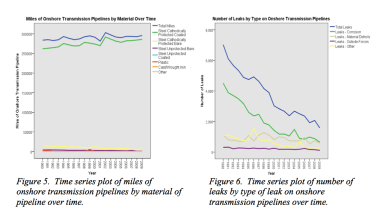
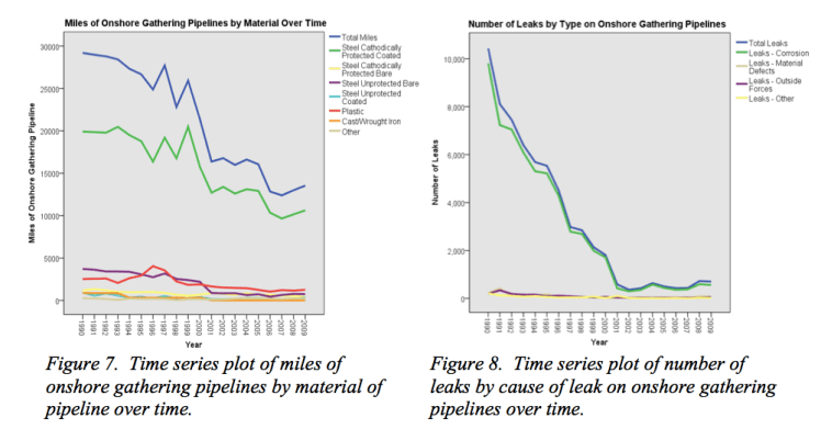
Time series plots are used to evaluate natural gas pipelines and leaks over time. A time series plot of miles of onshore transmission pipelines is shown in Figure 6. Each line on the graph represents a type of material of onshore transmission pipelines. The most common of which is cathodically protected coated steel. Figure 7 shows the sum of number of leaks over time on onshore transmission pipelines for each year.

The total miles of pipelines only increases slightly over time, indicating there are a few new pipelines, but mainly those being replaced. Sum of leaks, total number of leaks, and leaks from corrosion go down in a similar fashion. This decrease could be from replacing old pipelines that have corroded and also with the advancement of better materials that are less susceptible to corrosion.

Time series plots for gathering onshore pipelines in Figure 7 and Figure 8 are compared against the transmission onshore plots. Steel cathodically protected coated makes up the majority of all onshore gathering pipelines, but these decrease over time as seen in Figure 7. Total miles of pipeline fluxuate greatly, for example, in 1997 there were 27,714 miles of onshore gathering pipelines, which dips down to 22,798 in 1998, and then goes back up in 1999 to 25,917 miles before dropping off. Some reasons for this fluxuation could be pipelines being repaired during that year, gas drilling locations change, companies closing or no longer using the gathering pipelines, or incorrect recording in the data. Along with the drop in miles of pipeilne seen around 1999-2001 a significant drop in leaks occurs from 1990 to 2001.

Onshore and offshore pipelines are exposed to different habitats and therefore were looked at seperately when invsetigating leaks. Figure 9 shows that number of offshore transmission pipelines decrease over time, however leaks on offshore transmission pipelines in Figure 10 fluctuate greatly over the 19 year span.

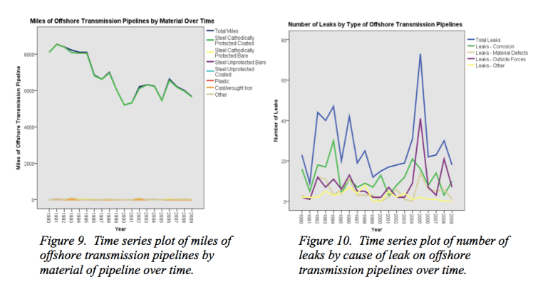
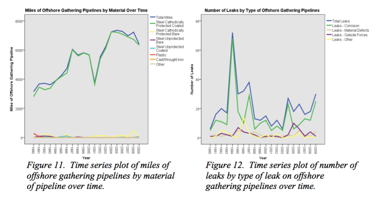
The number of offshore gathering pipelines increases over time (as seen in Figure 11), unlike onshore gathering pipelines. This makes us believe that some gathering pipelines were once being recorded onshore is now being recorded offshore. The number of leaks occurring on offshore gathering pipelines over the 19 years seems to also fluctuate as does onshore transmission pipelines. Figure 10 and Figure 12 show the number of leaks by cause of leak over time for offshore transmission pipelines and offshore gathering pipelines respectively. These figures show that the majority of leaks on these types of pipelines are from corrosion; however they also show fluctuations in all types of leaks. For example in Figure 10 there is a sharp increase in leaks from outside forces that occurred in 2005, which could be attributed to leaks caused from Hurricane Katrina.

4.3 REGRESSION ANALYSIS; TRANSMISSION DATA

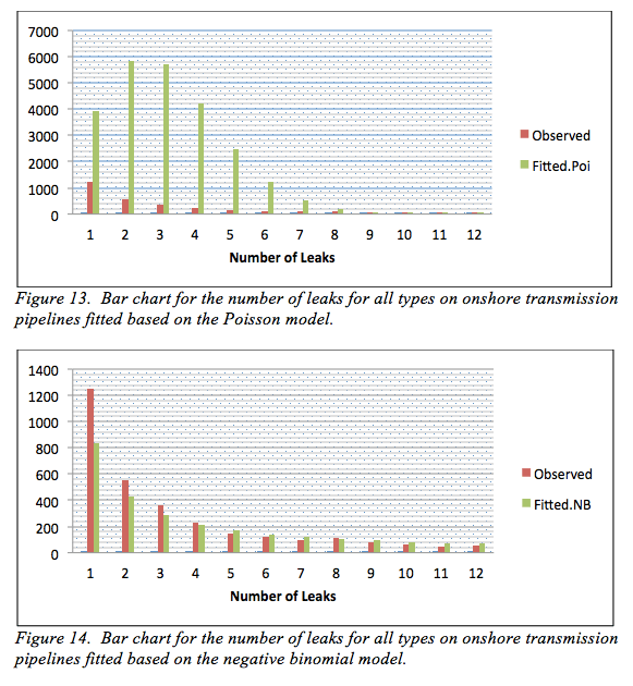
The outcome variables that were analyzed are the number of leaks for each cause. The number of leaks for all types of on onshore transmission pipelines range from 0 to 1550, indicating larger to smaller frequencies. In order to perform the regression analysis, we first need to find the appropriate model for the number of leaks. A bar chart for the number of leaks for all types of on onshore transmission pipelines is fitted based on the Poisson and negative binomial models and presented for only data ranging from 1 to 12 in Figures 13-14, respectively. These figures clearly show that the negative binomial model is much better fit compared to the Poisson model. Further, this data set is analyzed based on the descriptive statistics and goodness-of-fit of the both models and the results are provided in Table 1. The descriptive statistics in Table 1 show that the observed variance for the number of leaks is much larger than its mean, indicating a violation of the Poisson model assumption. Moreover, the confidence interval for dispersion in Table 1 shows that the number of leaks is significantly over-dispersed, which supports that the negative binomial would be better model for the number of leaks. This is also supported by the goodness-of-fit results in Table 1. Thus we conclude that the negative binomial model is more appropriate than the Poisson model.

Descriptive Statistics

Leaks Data	Size	25552
	mean	2.948732
	variance	922.7385
Estimation and Inference
NB Model	Estimates	St. Errors	95% Confidence Intervals
Mean	2.949	0.094	(2.764, 3.133)
Dispersion	25.583	0.461	(24.679, 26.487
Goodness-of-fit
Models	-2logL	AIC	BIC
NB	545095.9	545097.9	545106
Poisson	509116.2	509120.2	509136.5

Table 1: Descriptive statistics, estimates, and goodness-of-fit statistics for the number of leaks for all types on onshore transmission pipelines

The negative binomial regression model with the log link function follows the model equation:

ln(µ)= α + β₁X + β₂X + β₃X…,

where µ = E(Y) and β₁, β₂, β₃… are unknown parameters. This means the expected value of Y is E(Y)=µ=e^α * e^β1X1 * e^β2X2 * e^β2X2….

To find the predicted probability of number of leaks we can use the equation:

P(Y=y) = * (1-p)^r* p^k.

4.3.1 ONSHORE TRANSMISSION PIPELINE ANALYSIS

There were 25,552 data records within the transmission data set, 19,903 of which contained onshore transmission pipelines, which were analyzed. Seven data points from transmission onshore pipelines were removed for having extremely high leak rates. These rates were so high they seem like an input error. For example, one of the entries removed contains one mile of transmission onshore pipeline and 15 leaks. Sixteen records claim to have leaks on onshore pipelines; however that company does not record having any onshore pipelines for that year. These records are also removed. From this data set outliers and extremes are removed using 3 standard deviations from the mean as outliers and 5 standard deviations from the mean as extremes. This was done because the negative binomial regression model created on the full data set was extremely inaccurate and not significant. Removing all of these data records creates a data set with 18,788 records that the following regression models are performed on.

A negative binomial regression is performed on the data for each cause of leak. These target variables are leaks from corrosion, leaks from material defects, leaks from outside forces, leaks from other, and all leak types. Input parameter variables include the number of miles of: steel cathodically protected bare, steel cathodically protected coated, steel unprotected bare, steel unprotected coated, cast wrought iron, plastic, and other. Miles of pipeline by diameter were also investigated by negative binomial regression including miles of transmission onshore pipelines with diameter unknown, diameter < 4″, diameter 4″ – 10″, Diameter 10″ – 20″, diameter 20″ – 28″, and diameter > 28″. The models built to predict leaks are compared against each other using their average absolute residuals. The residual equals the absolute value of the predicted number of leaks minus the actual number of leaks. The average absolute residual tells us on average how far away the predicted value is from the actual value.

Some variables describing miles of pipe by diameter are significant in the model; however the models that contain these variables have larger average absolute residuals when compared to those models with only miles of material type. For this reason miles of pipeline by diameter variables are removed from the final model. The model with the lowest average absolute residual is found in Table 2 for each cause of leak. These models were built using a training set of 75% of the data and a test set of 25% to assess the quality of the regression analysis. The predictor variables or inputs are miles of pipeline by material type. These materials are steel cathodically protected bare, steel cathodically protected coated, steel unprotected bare, steel unprotected coated, cast wrought iron, plastic, and other. A weight field was used to account for total miles of onshore transmission pipelines for that company. A negative binomial distribution with a log link function was used with a hybrid parameter estimation method and a Pearson-chi-squared scale parameter. The model coefficients for each parameter are seen in the columns for each type of leak listed across the top in Table 2. Those starred (*) coefficients are deemed significant within the regression with an alpha level of 0.05. The italicized parameters, scale, negative binomial, and residuals, do not affect the regression equation but are looked at for model quality.

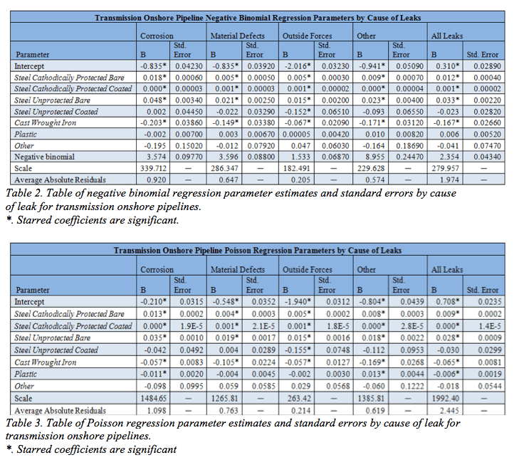
Analyses were performed separately for each target field (each cause of leak) and were leaks from corrosion, material defects, outside forces, other, and all leaks. The regression models above fit into the equation:

Ln(leaks) = Intercept + b₁(Steel Cathodically Protected Bare) + b₂ (Steel Cathodically Protected Coated) + b₃ (Steel Unprotected Bare) + b₄ (Steel Unprotected Coated) + b₅ (Cast Wrought Iron) + b₆ (Plastic) + b₇ (Other).

This implies the following:

Expected Number of Leaks = e^Intercept * e^{b1*Steel Cathodically Protected Bare} * e^{b2*Steel Cathodically Protected Coated} * e^{b3*Steel Unprotected Bare} * e^{b4*Steel Unprotected Coated} * e^{b5*Cast Wrought Iron} * e^b6*Plastic * e^b7*Other.

The fitted equation for leaks from corrosion is:

Ln(leaks) = -0.835 + 0.018*(Steel Cathodically Protected Bare) + 0.0*(Steel Cathodically Protected Coated) + 0.048*(Steel Unprotected Bare) + 0.002*(Steel Unprotected Coated) + -0.203*(Cast Wrought Iron) + -0.002*(Plastic) + -0.195*(Other).

The estimated coefficients listed can be interpreted by saying for each one-unit increase in cast wrought iron the expected log count of the number of leaks from corrosion decrease by 0.203 leaks.

Those coefficients with larger positive-values increase the number of leaks. For example, the equation predicts a company with 100 miles of onshore transmission pipelines made of steel cathodically protected bare to have 4.53 leaks where as if the 100 miles of pipeline were made of steel unprotected bare the predicted number of leaks would be 36.97. These predictions are the result of the following equations:

Leaks = e^0.310 * e^0.012*100= 4.53 leaks, for 100 miles of steel cathodically protected bare.

Leaks = e^0.310 * e^0.033*100= 36.97 leaks, for 100 miles of steel cathodically protected bare.

By comparing the coefficients of one material to another, one can see which materials cause more leaks. Since corrosion was the cause of most leaks, the material best used to prevent corrosion is of interest. Cathodic protection and coating are expensive procedures to ensure the pipeline’s integrity. This regression shows that out of the four types of steel, cathodically protected coated performs the best. The next best type of steel is unprotected coated. Cathodically protected bare still outperforms unprotected bare, which is predicted to have the most leaks. This confirms that the cathodic protection and coating used to protect the pipelines from corrosion does work. The coefficient for steel cathodically protected coated is not much different from steel unprotected coated, and the low number of leaks may be contributed mainly to the coating and not the cathodic protection. However, when comparing cathodically protected bare and unprotected bare pipelines the former does perform better than its unprotected counterpart. Comparing these to the other materials, the coefficient for cast/wrought iron predicts the least leaks, followed by other materials, and then plastic. All three of these materials produce lower leak predictions then any of the types of steel.

Next to the coefficients in the tables are the matching standard error which measures the amount of sampling error in the coefficient. These standard error values tell us how much the estimate is likely to vary from the parameter. Coefficients with high standard errors could potentially not be very accurate as it gives the coefficient a greater spread. Table 2 shows the regression output with the coefficients and their respective standard error values. This table implies that pipelines made of other materials have a higher standard error. This could be because there are less data points that contain pipelines made of other materials, and there are a variety of different kinds of materials within that category, some of which perform well and some not so well. For onshore transmission pipelines, other and cast wrought iron pipelines have negative coefficients that predict the least amount of leaks, but only the cast wrought iron coefficient is significant. This is because other has a standard error of 0.15 which is much higher than the standard error of cast wrought iron. Although cast wrought iron and other seem similar in corrosion leak effectiveness when comparing coefficients, it is also important to take their associated standard error into account. The p-value of the regression determines if the coefficient is significant with the associated standard error value. This is why coefficients of the same value could or could not be significant.

In a Poisson model dispersion is constrained to zero. In the negative binomial model, the dispersion coefficients are all greater than zero which makes it more appropriate for over-dispersed data than the Poisson model. An estimate greater than zero suggests over-dispersion, and an estimate less than zero suggest under-dispersion, where a binomial model may be appropriate. Poisson regression models are performed on the same data in order to compare both methods. The coefficients from the output can be seen in Table 3.

By comparing the residual values between the Poisson and negative binomial regressions, it is seen that the latter performs better. That is, the negative binomial regression models were more accurate.

A scatterplot of actual number of leaks versus predicted number of leaks (from the negative binomial regression model) is used to examine the effectiveness of the regression model. This is done for leaks from all causes and can be seen in Figure 15. Most of the leaks are concentrated around zero, and then increase from there. As the number of leaks increases, dispersion increases.

4.3.2 ONSHORE GATHERING PIPELINE ANALYSIS

Onshore gathering pipelines are analyzed separate from onshore transmission pipelines as discussed above. Both of these pipelines are onshore, however gathering pipelines carry unprocessed gas, which effects pipeline integrity differently.

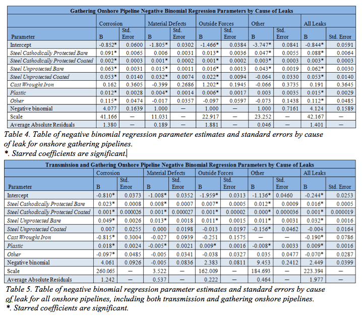
After removing all incorrect data, data with no onshore gathering pipelines, and removing outliers, the data set used in the analysis contains 7,230 records. The same negative binomial regression is performed on this data for onshore transmission pipeline data. Table 4 contains the summary of the regression models built.

Steel cathodically protected coated outperforms all materials in leaks from corrosion, as seen in onshore transmission pipelines. This material is the most popular material in both transmission onshore and gathering onshore pipelines as investigated in the time series charts in Figures 5 and 7. Cast wrought iron pipelines, which perform well in the transmission onshore pipeline regression in Table 2, performs very poorly in the gathering pipelines. This may be due to the corrosive compounds in untreated gas reacting with cast wrought iron, which causes leaks.

4.3.3 ALL ONSHORE PIPELINE ANALYSIS

Both transmission and gathering onshore pipelines were added together to be analyzed because separately the sample sizes were too small. The data set contained 25,552 data entries to start. Companies that had no onshore pipelines were filtered out. Data was flagged for having extremely high leaks per mile rate seemed like errors and were removed. The final data set had 24,253 valid entries. From here outliers and extremes were removed using 3 standard deviations from the mean as outliers and 5 standard deviations from the mean as extremes, which left with 22,693 records. The negative binomial regression was then used on this trimmed data set. The regression coefficient output is shown in Table 5. Similar associations between coefficients of materials can be seen in all onshore pipelines, transmission and gathering, as in transmission onshore pipelines found in Table 2.

4.3.4 ALL OFFSHORE PIPELINE ANALYSIS

Offshore pipelines are “defined in the Code of Federal Regulations as a pipeline that lies beyond the low water mark of the coast of the United States that is adjacent to the open seas” (PHMSA). States surrounding the great lakes once had offshore pipelines beneath the lake however in 2002 the federal law banned this. Currently only Michigan has pipelines below Lake Michigan, however these all originate from onshore locations. Many other coastal states have federal and state restrictions on offshore drilling. While analyzing offshore pipelines it was seen that some landlocked states recorded having some. Although offshore pipelines are clearly defined, “There are still many possible interpretations (whether correct or not) for what data is being requested. All this could result in someone reporting a river or lake crossing as offshore piping even though offshore is supposed to be on the outer continental shelf” (Miller). Because of this it is important to be careful with landlocked states that have offshore pipelines.

Only 10.5% of the data or 2,689 entries contain some form of offshore pipeline. These were categorized geographically by the state they operate from and also from which body of water they are most closely associated with. New variables were recorded for analysis of offshore pipelines to compare locations, which are state of operation offshore ocean (including Pacific Ocean, Gulf of Mexico, Atlantic Ocean, Great Lakes, and Land-locked) and state of operation offshore area (Pacific Ocean, Gulf of Mexico, and Other).

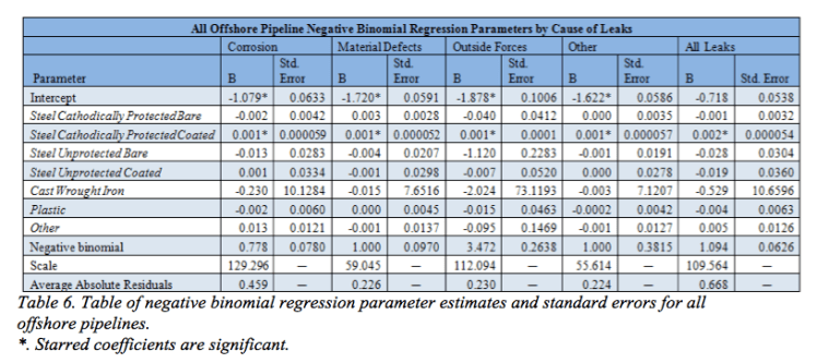
Transmission offshore and gathering offshore pipelines were combined to form one data set because of the low number of records. Outliers were not taken out of the data set because doing so removed almost all data that was not zero. When building the previous regression models, without removing outliers the models were extremely inaccurate, but in this case the outliers were not as extreme and the model performed fine when including them. Only 2,645 records were used in the analysis to form the regression output seen in Table 6. The only statistically significant material found in this regression output is steel cathodically protected coated, which is the most commonly used material. Steel unprotected bare has a coefficient of -0.013 for corrosion, which means that it predicts less leaks on this material compared to all others; however this coefficient is not significant so we cannot form any conclusions. A reason for most of the coefficients not being significant is because there is not enough data for significance to be determined.

4.3.5 OFFSHORE GATHERING AND OFFSHORE TRANSMISSION PIPELINE ANALYSIS

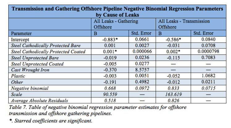
There are 961 records containing offshore transmission pipelines, and 1,893 records with offshore gathering pipelines. Since there were few records, and even fewer leaks, some types of pipelines do not have enough data to regress on. For this reason only total leaks were used as a response in the regression analysis for each offshore transmission and offshore gathering pipelines. It can be seen in Table 7 that there was not enough offshore transmission pipelines made of steel unprotected coated or cast wrought iron to be included in the analysis. Steel cathodically protected coated again is the only variable seen to be significant in both of these analyses because it is the only one with a low enough standard error and enough observations to support it.

Transmission and Gathering Offshore Pipeline Negative Binomial Regression Parameters by Cause of Leaks
	All Leaks – Gathering Offshore		All Leaks – Transmission Offshore
Parameter	B	Std. Error	B	Std. Error
Intercept	-0.883*	0.0661	-0.586*	0.0840
Steel Cathodically Protected Bare	0.001	0.0027	-0.031	0.0708
Steel Cathodically Protected Coated	0.001*	0.000066	0.002*	0.0000798
Steel Unprotected Bare	-0.019	0.0236	-0.115	0.7083
Steel Unprotected Coated	-0.005	0.0277	―	―
Cast Wrought Iron	-0.370	8.5757	―	―
Plastic	-0.003	0.0051	-0.052	1.0682
Other	-0.191	0.4982	-0.012	0.0211
Negative binomial	0.668	0.0972	0.833	0.0715
Scale	90.559	―	163.619	―
Average Absolute Residuals	0.518	―	0.826	―

DISTRIBUTION DATA ANALYSIS

The distribution pipeline data contains information on both main and service pipelines which are both found solely on land. Although there are a large number of service pipelines, these generally are a smaller diameter, carry less gas, operate under lower pressure, and travel for shorter distances. While main pipelines were recorded in miles, service pipelines are recorded in number of pipelines. One service pipeline could be one foot or one mile; the length is unknown in this study. This makes it hard to analyze and compare between pipeline materials and companies. Because of this non-uniform measurement, we concentrate on main distribution pipelines in this study. Excel files were obtained for each year from 1990 to 2010, which were merged together using Microsoft Access to create one large data set containing all distribution data including main and service pipelines which is analyzed below. A list of the original variables found in this data set can be seen in Appendix B.

5.1 DISTRIBUTION PIPELINE DATA CLEANSING

In the initial data set there were 30,612 data entries over the years 1990 to 2010. 100 duplicate cases were removed. Four hundred and ninety two out of 30,514 data points were missing state of operation variable. 97.0% of the 492 missing data points in the state of operation field were replaced with a valid state of operation record present in the same companies that had other listings with a valid entry. 3.0% of the 492 were unable to be determined and the missing state of operation variable was replaced with the state variable. It is possible that these assumed changes were incorrect but due to the small number of such errors would have negligible impact on the overall data for state of operation.

Some companies that reported miles of pipeline reported blank values instead of zeros for some of the materials. The total miles of pipeline may have been calculated by adding all of the non-missing recorded values, or it could have been recorded separately by the company. This means that total miles of pipeline could be total miles or total miles of non-missing pipeline (everything that was recorded). Over 97% of the entries in each number of miles of each material variable contain zero miles of pipeline. The cells that contained missing values were replaced with zeros so they would not be considered missing, and other variables could be calculated more easily from it. Three cells were missing data in the variable total miles of main pipeline and were replaced with the calculated sum from the miles of main for each material. The rest of the miles of main pipeline for each material were replaced with a zero if it was missing, which did not account for much of the data. Only nine values were missing and replaced with zeros in main steel unprotected coated, 11 from main steel cathodically protected bare, 14 from main steel cathodically protected coated, 167 from main cast wrought iron, 187 from ductile iron, 190 from copper, 192 from other_1, and 1,526 from other_2.

There were some cases where the total miles of main pipelines for each company did not equal the sum of the miles for each material. This may be due to company error or erroneously replacing a missing value with a zero. This difference was usually small and was not changed. The total miles of pipeline used in the analysis was the one recorded by the company and not the calculated value. In two cases this recorded main total miles was missing and was replaced with the calculated value.

Plastic was split up into three different types; PVC, PE, and ABS. The total of the different types equaled the recorded total miles of plastic, most of which was PE plastic. Separately the three types were not always significant, total plastic was used in that analysis.

In miles of pipeline for each material there were missing values. It was checked if the values are missing the total of all diameters still equaled the total miles when replaced with zero. In these cases from main and service pipelines all variables of miles of pipeline for each diameter and material were replaced with zero.

Number of leaks by type was seen in both main and service pipelines and there were a few missing values, which were all replaced with zero since it had been seen that some companies did not record the value if the value was zero. 47 companies that had zero miles and zero service pipelines were removed since they do not add any additional knowledge to the data set, and 155 duplicate cases were removed. The final data set containing 30,441 data entries was used in the analysis of the distribution data.

5.2 EXPLORITORY DATA ANALYSIS; DISTRIBUTION DATA

A map coding the total miles of main distribution pipelines in 2010 by state can be seen in Figure 16, which shows that the states with the largest number of pipelines were California, Texas, Illinois, Ohio, and Michigan. This map differs from the total miles of onshore transmission pipelines where southern states such as Louisiana, Kansas, Oklahoma, and Mississippi are replaced by Illinois, Michigan, New York, and Pennsylvania. Since these pipelines distribute the gas from where the transmission pipelines bring it, the map shows us where the gas is transported to.

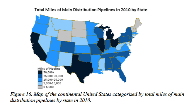
The rate of leaks per mile of main distribution pipelines in 2010 can be seen in Figure 17, which makes it evident that the higher percentage of leaks is concentrated in the northeast and then through the south. This association is important to keep in mind when looking at the data in the later analysis.

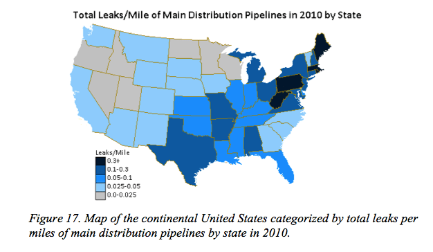
Figure 18 shows the miles of main pipeline by material over time. Steel cathodically protected, along with plastic, made up most of the miles of main pipeline. As the amount of main pipeline continues to grow, it is evident that over the last 11 years plastic pipelines have also continued to increase, which shows that plastic is the preferred material as it is the only material of main pipeline that has visibly grown.

Figure 19 shows the number of leaks over time broken up by material. It is evident that the total numbers of leaks have decreased over time, even though the miles of pipelines continue to increase. This implies that methods of repairing and installing new pipelines have improved. Old pipelines have been replaced with new ones and new pipelines are of better quality or are less prone to leaks. Most causes of leaks, including leaks from corrosion, the most common type, seem to be declining over time; however leaks from material defects have shown an increase in the past 10 years. These leaks from material defects are the fault of the manufacturer and are probably due to faulty material.

Location of pipeline was looked at to see if there was a significant difference in pipeline leaks per mile in that area. While looking at region, division, and geographic groups, some of these are shown to be significantly different than others with respect to leaks and some are not. To simplify this geographical comparison, two temperature regions were compared: seasonal (North) versus temperate (South). There was a significant difference in some causes of leaks between the two geographical temperature areas. To test this, an independent sample t-test was used to compare seasonal and temperate regions for each cause of leak per total miles and in many cases equal variance is not assumed. P-values less than 0.05 indicate a significant difference. In Table 8 the summary of the leaks by cause and region are seen along with the p-value of the comparison. It is seen that temperature has a significant effect (all using a 2-sided test) on leaks from third party damage, leaks from construction defects, leaks from material defects, and leaks from other causes. All of these variables were compared using rates of leaks per mile.

It was seen that leaks from third party damages had a significantly higher likelihood of occurring in temperate regions. This goes against what we would expect because the study previously discussed above (“Risk-based,” 2001) claims that more vandalism cases are recorded in populated areas such as the Northeast while this analysis indicates that there are actually more leaks per mile from third party damages in the southern portions of the United States.

These geographical associations of leaks between areas may be coincidental. To investigate this concern the difference between numbers of leaks is analyzed by year. Third party damages were significantly higher in the temperate region compared to seasonal region consistently throughout every year. Leaks from construction defects and material defects have lower leak rates for temperate region, but these are not always significant between each year. Leaks from other causes are always higher in the seasonal region but this is not significant for every year.

The scatterplots of miles of pipeline versus number of leaks are examined for leak type to visually see if there are clusters between the hot and cold temperature regions as shown in Figure 20. One would expect as the miles of pipeline increases, the number of leaks would also increase, but this is not always the case especially within the data since it follows a negative binomial distribution as discussed previously and seen in Figures 13 and 14. Southern states shown in red have the highest miles of pipelines which are expected. While most of the data is seen from zero to 10,000 miles of pipelines and less than 1,000 leaks, there is a cluster of northern states that have a high number of leaks from corrosion even though they have few miles of pipelines. These clusters can be looked at to identify what is going on within these groups.

5.3 REGRESSION ANALYSIS; MAIN DISTRIBUTION DATA

The data set used to analyze main distribution pipelines starts with 30,441 records of which 30,123 contain main pipelines. Outliers are removed from the data set using 3 standard deviations from the mean as outliers and 5 standard deviations from the mean are considered extremes, which leaves 28,402 records for the analysis.

A negative binomial regression model is fitted with a log link function. Hybrid parameter estimation is used with a Pearson chi-square scale parameter, which measures dispersion when divided by the degrees of freedom. Setting the scale parameter to zero does not affect or change the parameter coefficients in any way. A weight field of total miles of main pipeline, utilized for the standardization of variables, is used in the regression analysis to account for companies having different lengths of total pipelines.

This negative binomial regression is used to model leaks from corrosion, leaks from third party damage, leaks from outside force, leaks from construction defects, leaks from material defects, leaks from other causes, and all leaks. The regression parameter coefficients, B, are given in the table below for each of these analyses. Material Other_2 is left out of the regression because its infrequency and lack of significance in all of the models.

A regression model is formed for each cause of leak and the summaries of the regression analysis coefficients (b_n values) for each cause of leak are summarized in Table 9.

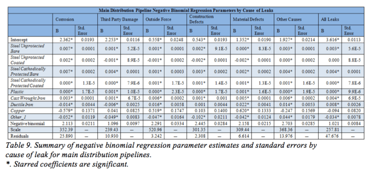
The fitted equation for leaks from corrosion is:

Ln(leaks)= 2.384 + 0.007*(Miles Steel Unprotected Bare) + 0.002*(Miles Steel Unprotected Coated) + 0.007*(Miles Steel Cathodically Protected Bare) + 0.0* (Miles Steel Cathodically Protected Coated) + 0.0*(Miles Plastic) + 0.003*(Miles Cast Wrought Iron) – 0.014*(Miles Ductile Iron) – 0.580*(Miles Copper) – 0.051*(Miles Other_1).

This equation can be solved to estimate the number of leaks for a company based on the miles of pipelines by material.

Over time steel cathodically protected coated has been replaced by pipelines made out of plastic, as seen in the time series plot in Figure 18. To understand why this has happened, the coefficients of the materials determine their effectiveness. Both steel cathodically protected coated and plastic seems to perform very similarly, they have coefficients around zero. By looking at the analysis, one type does not appear to be better than the other. We believe that plastic is used over steel cathodically protected coated because it is cheaper to manufacture and install. Materials such as copper and other_1 are seen to predict fewer leaks then plastic or steel cathodically protected coated, all of which are also statistically significant. Copper and other_1 are most likely not used as often as their less effective counterparts because of cost. This is especially seen in leaks from third party damage where copper has the highest coefficient of 0.041, which can be blamed on copper being expensive and sometimes stolen. Although more expensive materials could perform better, it would be more cost efficient to replace cheaper pipelines more frequently.

Figure 21 shows the scatterplot of predicted number of leaks versus actual number of leaks, which shows that the number of leaks versus the predicted number of leaks follows a pattern. The data is concentrated from zero to one hundred leaks, with more variation as the values extend from zero.

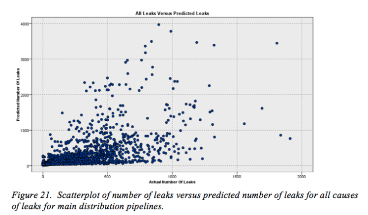
When trying to perform regression analysis on service distribution pipelines the results showed that the models were very poor and the predicted values were not close to the actual number of leaks. This may be due to the units are given by number of pipelines and not by miles. Since the results of the regression are not accurate they are not included in this paper.

DISCUSION

Steel cathodically protected bare is the most common material found in all types of transmission natural gas pipelines in this analysis. Being the most common material found, it is expected to hold up the best when related to leaks, is easy to use, or is most cost efficient. Although cathodically protected steal generally fairs better than its unprotected and bare counterparts, when compared against materials such as cast wrought iron, plastic, and other, the cathodically protected coated steel is not always the best option. In transmission onshore pipelines, the cast wrought iron coefficient predicts the least amount of leaks compared to the other materials. Discussed previously, these pipelines were favorable due to their resistance to corrosion however they are now being replaced with steel. Material categorized as other performs well in the analysis as having a coefficient that is both negative and significant at a 0.05 level, but sometimes has a high standard error. The problem with generalizing other material is that more than likely this means many different kinds of material, good or bad. This other material could include an old material that is no longer commonly in use, or new composite materials that are being looked at and becoming more popular. Plastic also shows a better option than steel when looking at leaks from corrosion of pipelines, however plastic pipelines are limited to those with less pressure. This is why plastic is more common in distribution pipelines where the pipes are carrying less gas and generally under less pressure. Plastic performs well in pipelines compared to its counterparts, possibly because the nature of the gas and how it reacts to metal materials. This performance depends however on the nature of the gas and the location of the pipeline.

Cast wrought iron is more susceptible to leaks in onshore gathering pipelines, in all types except material defects. This high rate of leaks from corrosion could be due to the raw form of the gas advancing the corrosion process. This material either does not stand up to its counterparts, or is older than the pipelines made of other materials that it is not holding up as well due to age. Onshore gathering pipes made of cast wrought iron should be examined to ensure that threats of a gas leak are not present. These pipelines should be replaced with more current materials.

Offshore pipelines are of different nature than onshore pipelines due to their environment. Total leaks for offshore transmission and offshore gathering pipelines are compared and seem to have similar trends. For all offshore pipelines, cast wrought iron and steel unprotected bare seem to perform the best (coefficients of -0.230 and -0.013 respectively), however they both contain large standard errors which make these estimates not significant. These pipeline materials could corrode slower when submerged in water, and are stronger than the other materials. Steel unprotected bare is seen to perform better than cathodically protected coated which is surprising and could be explained by the loss of cathodic protection when submerged in water, or the effect of the coating material.

Pipeline materials in distribution pipelines differ from those of transmission pipelines. The most common materials are cathodically protected coated steel and plastic. In more recent years, plastic has been replacing other materials, specifically cathodically protected coated. Comparing these two materials, they both seen equal with respect to leaks. Plastic may be the preferred method in recent years due to lower cost. When comparing plastic to the other materials it does not perform as well as pipelines made out of other or copper. Pipelines made of copper predict the least amount of leaks from corrosion and other causes. Although copper is least likely to corrode and has the least leaks overall, it has the highest rate of leaks from third party damages, outside forces, construction defects, and material defects when compared to all other materials. Copper proves to be a non-corrosive material, however with its inflexibility and high cost, other options prove to be preferred.

The associations and predictions found in this analysis could also be attributed to the idea that one material is more sustainable than another and therefore is not replaced as often as others. The analysis shows that plastic performs better than cast wrought iron in gathering onshore pipelines, but this could only be because plastic pipelines are expected to corrode faster and are therefore replaced more often. The difference between new and old pipelines in this analysis is not known and should be taken into consideration when interpreting these results.

6.1 CONCLUSIONS

By comparing regression models against each other, one can predict number of leaks by the materials they are composed of for each cause of leak. There is not one material that outperforms the others in all causes of leaks, and some materials work better in some environments then in others. It is necessary to consider the location of the pipeline and the nature of the gas being carried in order to accurately select the best material for that situation.

Companies can be reluctant in fixing or replacing old pipelines due to the nature of this work can cause more danger then the benefit of fixing them. By identifying which pipeline materials are more likely to cause leaks and for which reasons it gives the companies a starting point of what pipes may need to be surveyed, fixed, or replaced. The results of this analysis can improve safety control methods and evaluate the potential risk in preexisting pipelines. This study can reduce cost in prevention methods by focusing only on the methods needed for inspection and maintenance of high risk pipelines.

As talks of building new pipelines from Alaska to the continental United States, or tapping into shale deposits, the topic of pipelines are as important as ever. It is important to know which pipelines are most effective, safe, and prone to leaks, damages, and repairs to plan ahead in the construction process of new pipeline systems.

With people “depending on the smooth and uninterrupted operation of these lines, it is increasingly important to ensure the safe and failure-free operation of pipelines” (“Risk-based,” 2001). When looking at the repercussions of leaky pipelines all aspects must be considered including loss of product, environmental damage, health and safety of consumers, and financial consequences.

6.2 LIMITATIONS OF THE STUDY

The study is limited by the data that has been recorded and submitted online to the Pipeline and Hazardous Materials Safety Administration. Some of the data may have been recorded incorrectly or not recorded at all. For example it is known that the miles of pipelines installed during specific time periods is inaccurately measured for some of the data sets and net pipelines are recorded instead of overall new pipelines. Recording mistakes similar to this could have happened unknowingly for other variables as well.

Companies that operate over multiple states sometimes aggregate their data which could give false results when examining the leaks geographically if they are pooled into only one state.

Within the data, total miles of pipelines may not equal the sum of the miles of each type of pipeline given. There may be additional pipelines that are not accounted for in the subdivisions, or they may be recorded incorrectly.

Missing data from the companies could limit the models accuracy. Different years have different methods and variables that were reported. For example in the transmission data years 1990-2000 have similar formats for reporting variables however this format is changed for 2001-2009 and again in 2010. In these later years, types of leaks are broken down into smaller categories and there are also more variables about the pipelines themselves. This change requires combining variables for 2001-2009 for consistency over 1990-2010.

The data provided by the PHMSA has no formal data inspection and verification methods provided by the company. There is a chance that the “data was transposed when reported or when recorded. It may be possible that someone checked an incorrect box and PHMSA followed through when posting the data. Most importantly, one must look at the form instructions to see what PHMSA means by each term and what they are looking for in each piece of data. Unfortunately these instructions are not always as clear as one would think. There are still many possible interpretations (whether correct or not) for what data is being requested” (Miller). Until the PHMSA cleans up the data collecting recording process the provided data will be assumed to be true and valid for analysis purposes.

REFERENCES

About U.S. Natural Gas Pipelines- Transporting Natural Gas. (2007). Energy Information Administration. Retrieved April 20, 2012, from ftp://ftp.eia.doe.gov/pub/testdmr/Pipeline_a.pdf

Bryce, R. (2002). Pipe Dreams; Green, Ego, and the Death of Enron. New York, NY: PublicAffairs.

Census Bureau Regions and Divisions with State FIPS Codes. (n.d.). U.S. Census Bureau. Retrieved April 20, 2012, from http://www.census.gov/geo/www/us_regdiv.pdf

EXTERNAL CORROSION— Conclusion: Cased pipe segments could be less safe than uncased segments. (2009). Oil & Gas Journal, 107(15). Retrieved June 22, 2012, from http://www.ogj.com/articles/print/volume-107/issue-15/transportation/external-corrosionmdash-conclusion-cased-pipe-segments-could-be-less-safe-than-uncased-segments.html

Four-Color Problem. The Encyclopedia Of Science. Retrieved August 8, 2012, from http://www.daviddarling.info/images/USA_color_map.gif

Hallett, S., & Wright, J. (2011). Life without oil: Why we must shift to a new energy future. Amherst, NY: Prometheus.

History Zone. (n.d.). Pacific Gas and Electric Company. Retrieved May 3, 2012, from http://www.pge.com/microsite/safety_esw_ngsw/ngsw/more/history.html

Hovey, D. J., & Farmer, E. J. (1999). DOT stats indicate need to refocus pipeline accident prevention. Oil & Gas Journal, 97(11). Retrieved June 22, 2012, from http://www.ogj.com/articles/print/volume-97/issue-11/in-this-issue/general-interest/dot-stats-indicate-need-to-refocus-pipeline-accident-prevention.html

Inslee, J., & Hendricks, B. (2008). Apollo’s fire: Igniting America’s clean-energy economy. Washington, DC: Island Press.

Laney, P. (2002, July). Use of Composite Pipe Materials in the Transportation of Natural Gas. Retrieved June 12, 2012, from http://www.netl.doe.gov/technologies/oil-gas/publications/td/laney-paper.pdf

Maptech Support. (2003, October 08). Maptech. Retrieved August 14, 2012, from http://www.maptechnavigation.com/support/forums/messages.cfm?threadid=1101&CFID=2901702&CFTOKEN=69902104

Merriam-Webster. (n.d.). Retrieved June 9, 2012, from http://www.merriam-webster.com/

Miller, Kate. Message to Paul Pierson. 30 Mar. 2013. E-mail.

NaturalGas.org. (n.d.). NaturalGas.org. Retrieved April 20, 2012, from http://www.naturalgas.org

Natural Gas Delivery System Materials. (n.d.). American Gas Association. Retrieved June 13, 2012, from http://www.aga.org/Kc/aboutnaturalgas/additional/Pages/NGDeliverySystemMaterials.aspx

Nersesian, R. L. (2007). Energy for the 21st century: A comprehensive guide to conventional and alternative sources. Armonk, NY: M.E. Sharpe.

New London Texas School Explosion. (n.d.). Retrieved May 9, 2012, from http://www.newlondonschool.org/Articles15.htm

PHMSA – U.S. Department of Transportation Pipeline and Hazardous Materials Safety Administration. PHMSA – Data & Statistics – Distribution, Transmission, and Liquid Annual Data. Retrieved from http://www.phmsa.dot.gov/portal/site/PHMSA/menuitem.ebdc7a8a7e39f2e55cf2031050248a0c/?vgnextoid=a872dfa122a1d110VgnVCM1000009ed07898RCRD

Pierson, P. (2012, April 20). [E-mail to the author].

Risk-based model aids selection of pipeline inspection, maintenance strategies. (2001). Oil & Gas Journal, 99(28). Retrieved June 22, 2012, from http://www.ogj.com/articles/print/volume-99/issue-28/transportation/risk-based-model-aids-selection-of-pipeline-inspection-maintenance-strategies.html

Rui, Z., Metz, P. A., Reynolds, D. B., Chen, G., & Zhou, X. (2011). Regression models estimate pipeline construction costs. Oil & Gas Journal, 109(27). Retrieved June 22, 2012, from http://www.ogj.com/articles/print/volume-109/issue-27/transportation/regression-models-estimate-pipeline-construction.html

San Bruno Announces $70M Blast Settlement With PG&E. (2012, March 12). CBS San Francisco. Retrieved May 9, 2012, from http://sanfrancisco.cbslocal.com/2012/03/12/san-bruno-announces-70m-blast-settlement-with-pge/

Seismic Gas shut off valves-installation. (n.d.). Metro Retrofitting. Retrieved May 9, 2012, from http://www.gometroretro.com/retrofitting-services/automatic-gas-shut-off-valves/

Sunshine, W. L. (n.d.). 5 Types of Natural Gas Pipelines. About.com Energy. Retrieved June 19, 2012, from http://energy.about.com/od/drilling/a/5-Types-Of-Natural-Gas-Pipelines.htm

The Outer Continental Shelf. (n.d.). OCS Alternative Energy and Alternate Use Programmic EIS Information Center. Retrieved June 19, 2012, from http://ocsenergy.anl.gov/guide/ocs/index.cfm

Wan, J., Yu, Y., Wu, Y., Feng, R., & Yu, N. (2011, December 27). Hierarchical Leak Detection and Localization Method in Natural Gas Pipeline Monitoring Sensor Networks. National Center for Biotechnology Information. Retrieved June 12, 2012, from http://www.ncbi.nlm.nih.gov/pmc/articles/PMC3279208/

Worth, K. (2011, January 2). PG&E discovers additional leaks on natural gas pipelines. San Francisco Examiner. Retrieved May 9, 2012, from http://www.sfexaminer.com/local/bay-area/2011/02/pge-discovers-additional-leaks-natural-gas-pipelines

APPENDEX A:

APPENDEX B:

Table of Variables for Distribution Pipeline Data	Table of Variables for Transmission Pipeline Data
Year	Year
Company	Company
Street	Report ID
City	Operator ID
County	City
State	County
Zip	State
State of Operation	Zip
Main -Steel Unprotected Bare	State of Operation
Main – Steel Unprotected Coated	Gathering – Offshore – Steel Cathodically Protected Bare
Main – Steel Cathodically Protected Bare	Gathering – Offshore – Steel Cathodically Protected Coated
Main – Steel Cathodically Protected Coated	Gathering – Offshore – Steel Unprotected Bare
Main – Plastic	Gathering – Offshore – Steel Unprotected Coated
Main – Cast/Wrought Iron	Gathering – Offshore – Cast/Wrought Iron
Main – Ductile Iron	Gathering – Offshore – Plastic
Main – Copper	Gathering – Offshore – Other
Main – Other1	Gathering – Offshore – Systems Totals
Main – Other2	Gathering – Onshore – Steel Cathodically Protected Bare
Main – Total Miles	Gathering – Onshore – Steel Cathodically Protected Coated
Services -Steel Unprotected Bare	Gathering – Onshore – Steel Unprotected Bare
Services – Steel Unprotected Coated	Gathering – Onshore – Steel Unprotected Coated
Services – Steel Cathodically Protected Bare	Gathering – Onshore – Cast/Wrought Iron
Services – Steel Cathodically Protected Coated	Gathering – Onshore – Plastic
Services – Plastic	Gathering – Onshore – Other
Services – Cast/Wrought Iron	Gathering – Onshore – Systems Totals
Services – Ductile Iron	Transmission – Offshore – Steel Cathodically Protected Bare
Services – Copper	Transmission – Offshore – Steel Cathodically Protected Coated
Services – Other1	Transmission – Offshore – Steel Unprotected Bare
Services – Other2	Transmission – Offshore – Steel Unprotected Coated
Services – Total #	Transmission – Offshore – Cast/wrought Iron
Main – Steel – Diameter Unknown	Transmission – Offshore – Plastic
Main – Steel – Diameter < 2″	Transmission – Offshore – Other
Main – Steel – Diameter 2″ – 4″	Transmission – Offshore – Systems Totals
Main – Steel – Diameter 4″ – 8″	Transmission – Onshore – Steel Cathodically Protected Bare
Main – Steel – Diameter 8″ – 12″	Transmission – Onshore – Steel Cathodically Protected Coated
Main – Steel – Diameter >12″	Transmission – Onshore – Steel Unprotected Bare
Main – Steel – Diameter Total	Transmission – Onshore – Steel Unprotected Coated
Main – Ductile iron – Diameter Unknown	Transmission – Onshore – Cast/Wrought Iron
Main – Ductile iron – Diameter < 2″	Transmission – Onshore – Plastic
Main – Ductile iron – Diameter 2″ – 4″	Transmission – Onshore – Other
Main – Ductile iron – Diameter 4″ – 8″	Transmission – Onshore – Systems Totals
Main – Ductile iron – Diameter 8″ – 12″	Transmission and Gathering – Steel Cathodically Protected Bare
Main – Ductile iron – Diameter >12″	Transmission and Gathering – Steel Cathodically Protected Coated
Main – Ductile iron – Diameter Total	Transmission and Gathering – Unprotected Bare
Main – Copper – Diameter Unknown	Transmission and Gathering – Unprotected Coated
Main – Copper – Diameter < 2″	Transmission and Gathering – Cast/Wrought Iron
Main – Copper – Diameter 2″ – 4″	Transmission and Gathering – Plastic
Main – Copper – Diameter 4″ – 8″	Transmission and Gathering – Other
Main – Copper – Diameter 8″ – 12″	Transmission and Gathering – Total
Main – Copper – Diameter >12″	Gathering – Offshore – Diameter Unknown
Main – Copper – Diameter Total	Gathering – Offshore – Diameter < 4″
Main – Cast/wrought iron – Diameter Unknown	Gathering – Offshore – Diameter 4″ – 10″
Main – Cast/wrought iron – Diameter < 2″	Gathering – Offshore – Diameter 10″ – 20″
Main – Cast/wrought iron – Diameter 2″ – 4″	Gathering – Offshore – Diameter 20″ – 28″
Main – Cast/wrought iron – Diameter 4″ – 8″	Gathering – Offshore – Diameter > 28″
Main – Cast/wrought iron – Diameter 8″ – 12″	Gathering – Offshore – Diameter System Totals
Main – Cast/wrought iron – Diameter >12″	Gathering – Onshore – Diameter Unknown
Main – Cast/wrought iron – Diameter Total	Gathering – Onshore – Diameter < 4″
Main – Plastic PVC – Diameter Unknown	Gathering – Onshore – Diameter 4″ – 10″
Main – Plastic PVC – Diameter < 2″	Gathering – Onshore – Diameter 10″ – 20″
Main – Plastic PVC – Diameter 2″ – 4″	Gathering – Onshore – Diameter 20″ – 28″
Main – Plastic PVC – Diameter 4″ – 8″	Gathering – Onshore – Diameter > 28″
Main – Plastic PVC – Diameter 8″ – 12″	Gathering – Onshore – Diameter System Totals
Main – Plastic PVC – Diameter >12″	Transmission – Offshore – Diameter Unknown
Main – Plastic PVC – Diameter Total	Transmission – Offshore – Diameter < 4″
Main – Plastic PE – Diameter Unknown	Transmission – Offshore – Diameter 4″ – 10″
Main – Plastic PE – Diameter < 2″	Transmission – Offshore – Diameter 10″ – 20″
Main – Plastic PE – Diameter 2″ – 4″	Transmission – Offshore – Diameter 20″ – 28″
Main – Plastic PE – Diameter 4″ – 8″	Transmission – Offshore – Diameter > 28″
Main – Plastic PE – Diameter 8″ – 12″	Transmission – Offshore – Diameter System Totals
Main – Plastic PE – Diameter >12″	Transmission – Onshore – Diameter Unknown
Main – Plastic PE – Diameter Total	Transmission – Onshore – Diameter < 4″
Main – Plastic ABS – Diameter Unknown	Transmission – Onshore – Diameter 4″ – 10″
Main – Plastic ABS – Diameter < 2″	Transmission – Onshore – Diameter 10″ – 20″
Main – Plastic ABS – Diameter 2″ – 4″	Transmission – Onshore – Diameter 20″ – 28″
Main – Plastic ABS – Diameter 4″ – 8″	Transmission – Onshore – Diameter > 28″
Main – Plastic ABS – Diameter 8″ – 12″	Transmission – Onshore – Diameter System Totals
Main – Plastic ABS – Diameter >12″	Transmission and Gathering – Diameter – Unknown
Main – Plastic ABS – Diameter Total	Transmission and Gathering – Diameter – <4″
Main – Other1 – Diameter Unknown	Transmission and Gathering – Diameter – 4″ – 10″
Main – Other1 – Diameter < 2″	Transmission and Gathering – Diameter – 10″ – 20″
Main – Other1 – Diameter 2″ – 4″	Transmission and Gathering – Diameter – 20″ – 28″
Main – Other1 – Diameter 4″ – 8″	Transmission and Gathering – Diameter – > 28″
Main – Other1 – Diameter 8″ – 12″	Transmission and Gathering – Diameter – Total
Main – Other1 – Diameter >12″	Gathering – Offshore – Installed – Unknown
Main – Other1 – Diameter Total	Gathering – Offshore – Installed – Pre 1940
Main – Other2 – Diameter Unknown	Gathering – Offshore – Installed – 1940 to 1949
Main – Other2 – Diameter < 2″	Gathering – Offshore – Installed – 1950 to 1959
Main – Other2 – Diameter 2″ – 4″	Gathering – Offshore – Installed – 1960 to 1969
Main – Other2 – Diameter 4″ – 8″	Gathering – Offshore – Installed – 1970 to 1979
Main – Other2 – Diameter 8″ – 12″	Gathering – Offshore – Installed – 1980 to 1989
Main – Other2 – Diameter >12″	Gathering – Offshore – Installed – 1990 to 1999
Main – Other2 – Diameter Total	Gathering – Offshore – Installed – 2000 to 2009
Main – System Total – Diameter Unknown	Gathering – Offshore – Installed – Total
Main – System Total – Diameter < 2″	Gathering – Onshore – Installed – Unknown
Main – System Total – Diameter 2″ – 4″	Gathering – Onshore – Installed – Pre 1940
Main – System Total – Diameter 4″ – 8″	Gathering – Onshore – Installed – 1940 to 1949
Main – System Total – Diameter 8″ – 12″	Gathering – Onshore – Installed – 1950 to 1959
Main – System Total – Diameter >12″	Gathering – Onshore – Installed – 1960 to 1969
Main – System Total – Diameter Total	Gathering – Onshore – Installed – 1970 to 1979
Services – Steel – Diameter Unknown	Gathering – Onshore – Installed – 1980 to 1989
Services – Steel – Diameter < 1″	Gathering – Onshore – Installed – 1990 to 1999
Services – Steel – Diameter 1″ – 2″	Gathering – Onshore – Installed – 2000 to 2009
Services – Steel – Diameter 2″ – 4″	Gathering – Onshore – Installed – Total
Services – Steel – Diameter 4″ – 8″	Transmission – Offshore – Installed – Unknown
Services – Steel – Diameter >8″	Transmission – Offshore – Installed – Pre 1940
Services – Steel – Diameter Total	Transmission – Offshore – Installed – 1940 to 1949
Services – Ductile iron – Diameter Unknown	Transmission – Offshore – Installed – 1950 to 1959
Services – Ductile iron – Diameter < 1″	Transmission – Offshore – Installed – 1960 to 1969
Services – Ductile iron – Diameter 1″ – 2″	Transmission – Offshore – Installed – 1970 to 1979
Services – Ductile iron – Diameter 2″ – 4″	Transmission – Offshore – Installed – 1980 to 1989
Services – Ductile iron – Diameter 4″ – 8″	Transmission – Offshore – Installed – 1990 to 1999
Services – Ductile iron – Diameter >8″	Transmission – Offshore – Installed – 2000 to 2009
Services – Ductile iron – Diameter Total	Transmission – Offshore – Installed – Total
Services – Copper – Diameter Unknown	Transmission – Onshore – Installed – Unknown
Services – Copper – Diameter < 1″	Transmission – Onshore – Installed – Pre 1940
Services – Copper – Diameter 1″ – 2″	Transmission – Onshore – Installed – 1940 to 1949
Services – Copper – Diameter 2″ – 4″	Transmission – Onshore – Installed – 1950 to 1959
Services – Copper – Diameter 4″ – 8″	Transmission – Onshore – Installed – 1960 to 1969
Services – Copper – Diameter >8″	Transmission – Onshore – Installed – 1970 to 1979
Services – Copper – Diameter Total	Transmission – Onshore – Installed – 1980 to 1989
Services – Cast/wrought iron – Diameter Unknown	Transmission – Onshore – Installed – 1990 to 1999
Services – Cast/wrought iron – Diameter < 1″	Transmission – Onshore – Installed – 2000 to 2009
Services – Cast/wrought iron – Diameter 1″ – 2″	Transmission – Onshore – Installed – Total
Services – Cast/wrought iron – Diameter 2″ – 4″	Transmission and Gathering – Installed – Unknown
Services – Cast/wrought iron – Diameter 4″ – 8″	Transmission and Gathering – Installed – Pre 1940
Services – Cast/wrought iron – Diameter >8″	Transmission and Gathering – Installed – 1940 to 1949
Services – Cast/wrought iron – Diameter Total	Transmission and Gathering – Installed – 1950 to 1959
Services – Plastic PVC – Diameter Unknown	Transmission and Gathering – Installed – 1960 to 1969
Services – Plastic PVC – Diameter < 1″	Transmission and Gathering – Installed – 1970 to 1979
Services – Plastic PVC – Diameter 1″ – 2″	Transmission and Gathering – Installed – 1980 to 1989
Services – Plastic PVC – Diameter 2″ – 4″	Transmission and Gathering – Installed – 1990 to 1999
Services – Plastic PVC – Diameter 4″ – 8″	Transmission and Gathering – Installed – 2000 to 2009
Services – Plastic PVC – Diameter >8″	Transmission and Gathering – Installed – Total
Services – Plastic PVC – Diameter Total	Gathering – Onshore – Class 1
Services – Plastic PE – Diameter Unknown	Gathering – Onshore – Class 2
Services – Plastic PE – Diameter < 1″	Gathering – Onshore – Class 3
Services – Plastic PE – Diameter 1″ – 2″	Gathering – Onshore – Class 4
Services – Plastic PE – Diameter 2″ – 4″	Gathering – Onshore
Services – Plastic PE – Diameter 4″ – 8″	Transmission – Onshore – Class 1
Services – Plastic PE – Diameter >8″	Transmission – Onshore – Class 2
Services – Plastic PE – Diameter Total	Transmission – Onshore – Class 3
Services – Plastic ABS – Diameter Unknown	Transmission – Onshore – Class 4
Services – Plastic ABS – Diameter < 1″	Transmission – Onshore
Services – Plastic ABS – Diameter 1″ – 2″	Transmission & Gathering – Onshore – Class 1
Services – Plastic ABS – Diameter 2″ – 4″	Transmission & Gathering – Onshore – Class 2
Services – Plastic ABS – Diameter 4″ – 8″	Transmission & Gathering – Onshore – Class 3
Services – Plastic ABS – Diameter >8″	Transmission & Gathering – Onshore – Class 4
Services – Plastic ABS – Diameter Total	Transmission & Gathering – Onshore
Services – Other1 – Diameter Unknown	Leaks – Corrosion – Gathering – Onshore
Services – Other1 – Diameter < 1″	Leaks – Corrosion – Gathering – Offshore
Services – Other1 – Diameter 1″ – 2″	Leaks – Excavation – Gathering – Onshore
Services – Other1 – Diameter 2″ – 4″	Leaks – Excavation – Gathering – Offshore
Services – Other1 – Diameter 4″ – 8″	Leaks – Equipment and Operations – Gathering – Onshore
Services – Other1 – Diameter >8″	Leaks – Equipment and Operations – Gathering – Offshore
Services – Other1 – Diameter Total	Leaks – Material Defects – Gathering – Onshore
Services – Other2 – Diameter Unknown	Leaks – Material Defects – Gathering – Offshore
Services – Other2 – Diameter < 1″	Leaks – Natural Forces – Gathering – Onshore
Services – Other2 – Diameter 1″ – 2″	Leaks – Natural Forces – Gathering – Offshore
Services – Other2 – Diameter 2″ – 4″	Leaks – Other – Gathering – Onshore
Services – Other2 – Diameter 4″ – 8″	Leaks – Other – Gathering – Offshore
Services – Other2 – Diameter >8″	Leaks – Other Outside Forces – Gathering – Onshore
Services – Other2 – Diameter Total	Leaks – Other Outside Forces – Gathering – Offshore
Services – System Total – Diameter Unknown	Leaks – Corrosion – Transmission – Onshore
Services – System Total – Diameter < 1″	Leaks – Corrosion – Transmission – Offshore
Services – System Total – Diameter 1″ – 2″	Leaks – Excavation – Transmission – Onshore
Services – System Total – Diameter 2″ – 4″	Leaks – Excavation – Transmission – Offshore
Services – System Total – Diameter 4″ – 8″	Leaks – Equipment and Operations – Transmission – Onshore
Services – System Total – Diameter >8″	Leaks – Equipment and Operations – Transmission – Offshore
Services – System Total – Diameter Total	Leaks – Material Defects – Transmission – Onshore
Leaks – Corrosion – Mains	Leaks – Material Defects – Transmission – Offshore
Leaks – Outside Force – Mains	Leaks – Natural Forces – Transmission – Onshore
Leaks – Third Party Damage – Mains	Leaks – Natural Forces – Transmission – Offshore
Leaks – Material Defect – Mains	Leaks – Other – Transmission – Onshore
Leaks – Construction Defect – Mains	Leaks – Other – Transmission – Offshore
Leaks – Other Cause – Mains	Leaks – Other Outside Forces – Transmission – Onshore
Leaks – Corrosion – Services	Leaks – Other Outside Forces – Transmission – Offshore
Leaks – Outside Force – Services	Leaks – Gathering – On Federal Land – Offshore
Leaks – Third Party Damage – Services	Leaks – Gathering – On Federal Land – Onshore
Leaks – Material Defect – Services	Leaks – Gathering – Outer Continental Shelf
Leaks – Construction Defect – Services	Leaks – Transmission – On Federal Land – Offshore
Leaks – Other Cause – Services	Leaks – Transmission – On Federal Land – Onshore
Leaks – Scheduled for Repair	Leaks – Transmission – Outer Continental Shelf
Leaks on Federal Land Scheduled for Repair	Leaks – Gathering – Scheduled for Repair
Percent of Unaccounted for Gas	Leaks – Transmission – Scheduled for Repair
Date_of_Entry	AGA MEMBER
AGA_MEMBER
Miles of Main Installed – Unknown
Miles of Main Installed – Pre-1940
Miles of Main Installed – 1940-1949
Miles of Main Installed – 1950-1959
Miles of Main Installed – 1960-1969
Miles of Main Installed – 1970-1979
Miles of Main Installed – 1980-1989
Miles of Main Installed – 1990-1999
Miles of Main Installed – 2000-2009
Miles of Main Installed – 2010-2019
Miles of Main Installed – Total
Number of Service Installed – Unknown
Number of Service Installed – Pre-1940
Number of Service Installed – 1940-1949
Number of Service Installed – 1950-1959
Number of Service Installed – 1960-1969
Number of Service Installed – 1970-1979
Number of Service Installed – 1980-1989
Number of Service Installed – 1990-1999
Number of Service Installed – 2000-2009
Number of Service Installed – 2010-2019
Number of Service Installed – Total
Miles_of_Services
Date_of_Report
Number_of_Excavation_Damages
Number_of_Excavation_Tickets

Natalie Alexandra Sullo

Masters Project

Analysis of the U.S. Natural Gas Pipeline System With Respect to Leaks.

Leave a comment Cancel reply

Natalie Alexandra Sullo

Analysis of the U.S. Natural Gas Pipeline System With Respect to Leaks.

Share this:

Leave a comment Cancel reply