Natalie Alexandra Sullo

 

This project is used as practice for imputing missing data using the book “Discovering Knowledge in Data” by Daniel Larose. The analysis is created in SPSS Modeler.

The ‘ClassifyRisk – Missing’ dataset file was used and all missing values are imputed. This data set had 246 total records and 6 variables: marital status, mortgage, loans, risk, income, and age. There are missing (blank) and $null$ data in some of the variables. The following summarizes the variables and the location of the missing data:

Categorical variables:

Marital status- married, single, other (1 missing data points in record 19)

Mortgage- y, n (1 missing in record 8)

Risk- Good risk, bad loss (no missing or null records)

Continuous:

Income- continuous # (two $null$ data points in record 11 and 15

Age- continuous # (1 missing in record 11)

Loans- 1, 2, 3, (1 $null$ in record 7)

The first step that was performed was taking the Z-score standardization of the continuous variables. This standardization makes the variables have a more normal curve that is centered around zero. The equation for the Z-standardization is defined as:

Variable_z = Variable – mean (Variable) / SD (Variable)

This standardization is created using derive nodes for each of the variables and setting globals to create the mean and standard deviations of the entire data set. The end equation used is: variable-@global_mean(variable) / @global_sdev(income).

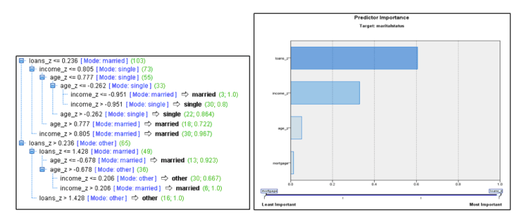
A CART model is then performed on marital status to predict the one missing record in the data set. The output from this model can be seen below. This output shows that loans, income, and age are the three most important factors in predicting marital status. Also given is the classification and regression tree that is used to predict the missing values.

From here a new variable is created titled marital status_total which gives the total of marital status data set and replaces the missing value with the predicted value from the above regression. This equation to form this data set is “If maritalstatus=”” then ‘$R-maritalstatus’ else maritalstatus endif”.

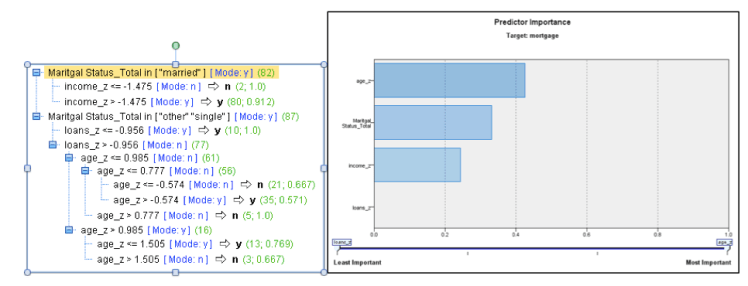
The missing values for mortgage are then predicted using the same CART model method. The classification and regression tree output is pictured below showing that the age, marital status, income, and loans are the four biggest predictors of mortgage. The predicted values replace the missing values and the complete variable name is titled mortgage_total.

Mortgage and marital status are then turned into flag dummy variables in order to be used in the regression model to predict continuous variables. Mortgage is made into martgage_yes since there is only yes and no values. Marital status is made into marital status_single and marital status_married since there is single, married and joint options. Regression models are ran with the target variable as the variable you are trying to impute values for. The response variable is not included in the regression and a stepwise regression model is performed to select the most significant variables. Income and age are both missing from observation number 11. In this case we will have to build a regression model without one of the predictor variables to predict the other. A regression model for age is performed first and the output is seen below. The variables loans_z, mortgage_yes, Marital Status_Married, and Marital Status_single are included in the regression, and income is left out. The regression equation that is give from the model is:

Predicted Age_z = 0.0008021*Loans_z + 0.3559*Mortgage_yes – 0.6039*Marital Status_married – 1.126*Marital Status_single + 0.3331

                      

 The Adjusted R squared of the model is seen as 0.198, which means that the model being built is not very good at creating the predictions; however the model is seen as significant having a p-value of 0.000, which is significant. A variable titled Age_z_all is created with the values of Age_z and the missing values are replaced with the predicted values of age_z.

A regression model is performed on income_z to produce the equations and output seen below. Put in the model was loans­­_z, morgage_yes, marital status_married, Marital Status_single, and age_z_all. In this model age is included with the predicted values in replace of the missing values. The model shows that loans are the most important predictor in the model. The adjusted R squared value is 0.291 which again is not very strong, but still seen as significant. The new variable with the replaced predicted values is titled income_z_all. The regression equation can be defined as:

Predicted Income_z = -0.5386*loans_z + 0.00722*mortgage_yes +0.1018*marital status_married – 0.6884*marital status_single – 0.1088*Age_z_all + 0.1688 

The regression of loans_z is performed using all the variables. The data file with the replaced missing values is saved as Loans_z_all.

Predicted Loans_z = -0.2494*mortgage_yes – 1.259*marital status_married – 1.76*marital status_single – 0.03*Age_z_all – 0.279*income_z_all +1.283

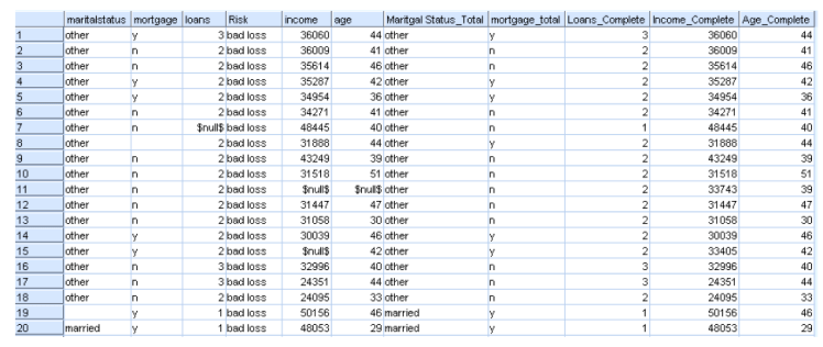
Loans_z_all, Age_z_all, and Income_z_all are all converted back to their original format and saved with the extension variable_complete. This is done with the derive node and the equation “round((Variable_z_all * @GLOBAL_SDEV(‘Variable’)) + @GLOBAL_MEAN(‘Variable’))”. The following table shows the original six variables along with the fields with the filled in missing values. All of the missing fields and their new values can be seen below.