Natalie Alexandra Sullo

 

Predicting The Response of High Yield Donors To Maximize Profit

 

EXECUTIVE SUMMARY

The Wounded Veterans of America (WVA) is a “a not-for-profit organization that provides programs and services for US veterans with injuries or disease”. The association raises money for veterans by direct mail fund raisers. The WVA keeps a database of everyone that has donated to the foundation at least once. The WVA is interested in improving the effectiveness of their direct mail marketing to maximize net revenue.  The data file provided (the training data set) includes 181,779 data points from a subset of 3.5 million donors and includes 34 variables. The data records consists of previous donors that have made there last donation 13-24 months ago (lapsing donors) and who have received the June 1997 renewal mailing. The two target variables are TARGET_B, if the donor responded to the promotion, and TARGET_D, the dollar amount of the responder’s gift. 1997 is used as the reference data in this analysis. The purpose of this analysis is to build a model predicting which prospective donors will in fact donate money. It is important to maximize total net revenue for the model, and in turn for the company. The validation file is used to build a model to predict which customers should be sent promotions. All the data was prepared and normalized before creating the model. Then a C5.0 classification model was used to predict TARGET_B while also offering propensity scores (the probability of the donor donating). TARGET_D was then predicted using a linear regression model. The estimated donation values found from the regression node were then multiplied by the propensity scores to create expected donation. This value was used in calculating overall profits by using the cost of mailing a promotion as $0.68. It was found that within the training file, the model predicted a total net profit of $65,905.65 which is a significant increase from the null model of send everyone a promotion. This same model predicts a net revenue of $3,126.35 on the validation data file. The prediction of those that will donate and who the promotion should be mailed to within this 10,000 record data set was predicted and the output saved. Using these multiple step models it is evident that complex associations can be found in predicting those customers that will donate and will increase donation revenues significantly.

 

DATA PREPARATION

 

The PVA training file used has 181,779 data points and 34 variables. A list of the variables, a summary of their definition taken from the given data dictionary, the output from an audit node on missing values, and methods of transformation can be found in figure 1.

Field	Field Description	Valid Records	Null/ White Space	Type of Transformation Used	New Variable Name or Type
AVGGIFT	Average dollar amount of gifts to date	181779	0	Natural Log
CARDGIFT	Number of lifetime gifts to card promotions to date	181779	0	Z-score
CARDPM12	Number of card promotions received in the last 12 months	181779	0	Z-score
CARDPROM	Lifetime number of card promotions received to date.	181779	0	Z-score
CONTROLN	Control number (unique record identifier)	181779	0	–
DOB	Date of birth (YYMM, Year/Month format.)	181779	0	Z-score	Age
DOMAIN	Urbanicity level of the donor’s neighborhood/Socio-Economic status of the neighborhood	177277	4502	–	Flag fields created
FISTDATE	Date of first gift	181779	0	SQ RT	FIRSTDATE_years
GENDER	Gender	176178	5601	–	Flag fields created
HIT	total number of known times the donor has responded to a mail order offer other than PVA’s	181779	0	Natural Log
HOMEOWNR	Home Owner Flag	139329	42450	–	Flag fields created
INCOME	HOUSEHOLD INCOME	141155	40624	Z-score
LASTDATE	Date associated with the most recent gift	181779	0	Z-score	LASTDATE_years
LASTGIFT	Dollar amount of most recent gift	181779	0	Natural Log
MAJOR	Flag major donor	546	181233	–	Flag fields created
MAXADATE	Unknown	181779	0	Z-score	MAXADATE_years
MAXRAMNT	Dollar amount of largest gift to date	181779	0	Natural Log
MAXRDATE	Date associated with the largest gift to date	181779	0	Z-score	MAXRDATE_years
MINRAMNT	Dollar amount of smallest gift to date	181779	0	Natural Log
MINRDATE	Date associated with the smallest gift to date	181779	0	Z-score	MINRDATE_years
NEXTDATE	Date of second gift	162744	19035	Z-score	NEXTDATE_years
NGIFTALL	Number of lifetime gifts to date	181779	0	SQ RT
NUMCHLD	Number of children	23442	158337	Z-score
NUMPRM12	Number of promotions received in the last 12 months	181779	0	Z-score
NUMPROM	Lifetime number of promotions received to date.	181779	0	Natural Log
RAMNTALL	Dollar amount of lifetime gifts to date	181779	0	Natural Log
RFA_2A	Code for the amount of the last gift	181779	0	–
RFA_2F	Number of gifts in the period of recency (13-24 months ago)	181779	0	Z-score
RFA_2R	Status of the donors- All lapsing donors	181779	0	–	Flag fields created
TARGET_B	Target Variable: Binary Indicator for Response to 97NK Mailing	181779	0	–
TARGET_D	Target Variable: Donation Amount (in $) associated with the Response to 97NK Mailing	181779	0	Natural Log
TIMELAG	Number of months between first and second gift	162744	19035	Natural Log
WEALTH1	Wealth Rating	96434	85345	Z-score
WEALTH2	Wealth Rating. 0-9, 9 being highest income group and zero being the lowest.	98364	83415	Z-score

Figure 1. Table of fields and their description found in the PVA Training File.

By examining the output from the audit node for all variables it is evident that there are some variables with missing records within the data. To resolve this problem all missing values were imputed. The process of how this is done is discussed below. The target variables TARGET_B and TARGET_D are not included in the models for imputing the data since they will not be present in future data.

RFA_2R is filtered out of the data set because all of the values are “L” for lapsing donor.

The variable Age was derived from the DOB variable. DOB was set up in the formal YYMM. The year is assumed to take place in the 1900’s making 19 the beginning two digits of the year number. For example the record that has a DOB of 3203 means that the person was born in March of 1932. Records with a DOB of only 2 values are assumed to be incorrectly recorded. Values with three numbers are believed to have a zero in front of the value for example 901 is actually 0901, having a date of birth of January of 1909. From this information we calculate age using a derive node and the if statement “If DOB> 99 Then 97- round(DOB / 100) Else undef”.  Using this formula to calculate Age rounds the value to discard the month and makes age to the closest year. All other values in this definition are made to a null field so they can later be imputed.

The variable gender is altered to replace missing and incorrect values. This is done using the if statement “If GENDER= “ ” or GENDER= “” or GENDER= “A” or GENDER= “C” Then “U” Else “GENDER” ”. This takes away any null, missing, or incorrect values and the final variable has only male, female, joint or undefined as possible responses. All missing, undefined, or incorrectly recorded (A or C) are recoded into “U” for undefined.

MAJOR is a flag variable with either X or a blank space as the value. This variable is recoded into a flag field with 1, if there once was an X, or 0 for a blank space.

NUMCHLD which contains discrete values 1-7 also has a majority of null fields. Since there are no zero values the null values are assumed to be zero and are replaced so there are no longer any missing values.

The variable FIRSTDATE_years is calculated from FIRSTDATE which tells us the years since the first time that member donated money. This version of the variable can be read and understood more easily while doing regressions by changing it from a date to a continuous value, years. The method to do this is the same as calculating Age from DOB. This was also performed on LASTDATE, MAXRDATE, MINRDATE, NEXTDATE, and MAXADATE all with a suffix of _years.

HOMEOWNER variable is made into the flag field HOMEOWNER_Y which made 1=homeowner and 0=unknown or missing.

The DOMAIN variable is split into two variables DOMAIN_1 and DOMAIN_2. This was done by using the equation “DOMAIN_1= substring(1, 1, DOMAIN)” and “DOMAIN_2= Substring(2, 1, DOMAIN)”. The missing values of these were then predicted using a CART model. Wealth1, Wealth2, and HIT are seen as the biggest factors in predicting DOMAIN_1 in the classification and regression tree.   Wealth1 is the most important factor in predicting DOMAIN_2. The predicted values from this model are used to replace the missing values within the variables.

The missing values in Income are predicted using a CART model. Although income is a continuous variable it is seen as being binned categories and is predicted using a regression tree. DOMAIN_2, Homeowner_Y, and Age are the biggest predictors used within the classification and regression tree for predicting Income.

Set to flag variables are made for Gender for _F, _M, _J, RFA_2A for _D, _E, _F, _G, DOMAIN_1 for _C, _R, _S, _T, and DOMAIN_2 for _1, _2, and _3.

Continuous variables were Z score standardized using the equation X- mean(X) /Standard Deviation(X). These variables, with the suffix of _z, along with the flag variables were used in regression models to predict the remaining continuous variables. The first regression model was built to predict the missing records in NEXTDATE_years_z. A select node is used to select only those records where there is a valid field for the variable being predicted and then a regression model is performed using a stepwise build method to see the best possible arrangement of variables into the analysis. The regression model is then run on this selection. The predicted values from this regression are then used to fill in the missing values within the variable. Regression models like this were performed for Age_z, TIMELAG_z, WEALTH_2 and WEALTH_1, in that order.

These new variables with imputed missing values are then returned to their original form by unstandardizing them and rounding when needed. This new data is exported into a new file and saved. This new file will be used throughout the project as the new data. The data with missing records is filtered out. This new data with the imputed values is then examined and the correct transformation for each variable is selected. Both continuous fields and ordinal fields that have a hierarchal relationship where order matters were standardized. This was done by examening histograms for each varaible for a variety of different transformations. The transform node was used to give an output for a variety of different options. The transformation that formed a distribution closest to normal was chosen for that variable. In figure 1 the variable name is stated along with the transformation chosen. Some variables were taken the natural logorithm, or square root transformations. It was found that some of the variables that were being normalized using a natural logorithm method had zero values which created errors after the transformation was perfomed. To prevent this 0.5 was added to the value of the variable and then taken the natural logorithm of (ln(X+0.5)). This is the case throughout the whole valiables life, however to short hand this in the variables the suffix of this new variable is still “_ln”. After these variables were transformed to a more normal distribution, the z-score standardization ( (X – Mean(X)) / Standard Deviation(X) ) was taken of all the variables.

An auto cluster node was performed on the data to test to see if clusering the data into groups would help in the analysis. The node build three cluster models. The twostep model with 5 clusters was chosen as the best cluster model for predicting TARGET_B. By using a cluster node it is my hope that it will produce groups that will help regression. These groups may separate one time donors, multiple donors, high value donors etcetera and aid in determening responders versus non responders. A twosetp model with 3 clusters was the best model built predicting TARGET­_D.

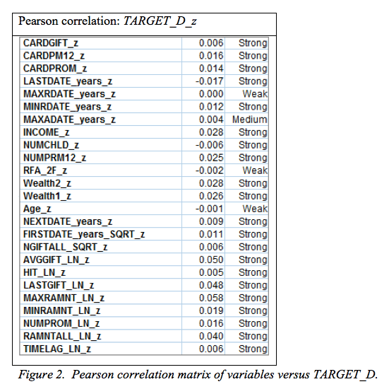
To compare the relationships between all of the variables, correlation matriz’s were created for all combinations. Most of the correlations between variables were seen as strong correlations. Below in figure 2 is the pearson correlation between TARGET­­_D and all continuous predictors. The correlations shown as week below will not be used in the regression model to create predictors of TARGET­­_D. These include standardized versions of Age, RFA_2F, MAXADATE_years, and MAXRDATE_years.

 

PROBLEM 1. PREDICTING TARGET

 

A model is to be built to predict TARGET_B. This value is either a 1, if the donor responded to the mail promotion, or 0, if the donor did not respond. In order to build a model with the best accuracy the data file is split up into a training data file and a test data file using a 70%-30% split respectively. This is done to build a classification model on the training data file and then test the predictions on the test data file. Using a partition node the data is split to form the training data file with 127,154 data points and a test data file with 54,625 data points.

Within the whole data set of 181,779 data records, 9,218 donors responded to the mailing (TARGET_B = 1), and 172,561 donors did not respond (TARGET_B = 0). Since only about 5% of the data is donors a null classification model would predict all TARGET_B = 0. This model would be useless as it would not help to predict those that would respond to the mailing. In this case it is necessary to balance the data. After the training data file is created a balance node is used to increase the 5% donors (TARGET_B = 1) to 6 times the amount and also decrease the non-donors (TARGET_B = 1) to 0.4 times the amount. It is chosen to increase the donor records and to get rid of some of the non-donors because only eliminating non-donors is eliminating a significant amount of the data and removing information from the data set. Duplicating donors is duplicating already existing data and no information is being lost. In the original training data set there are 120,780 non-donors and 6,374 donors. After the balance node there are around 48,300 non-donors and 38,200 donors. Every time the balance node is ran it re-balances so the values from this output will change. About 44% of the data in the training data file are donors. This will enable the regression model to predict both donors and non-donors for TARGET_B.

A C5.0 model is then ran on this balanced training data set to create a model to predict TARGET_B. The results from this model are then run through the test data set to ensure that the model is not giving false results by overtraining or memorizing the data set. To compare TARGET_B and predicted TARGET_B a matrix node is used. This shows us all true positives, true negatives, false positives, and false negatives. From this matrix we can use these values to calculate overall error rate and overall model accuracy in order to compare different models and choose the best model for predicting TARGET_B. These terms are defined below.

True Positive= Predicting TARGET_B=1 when TARGET_B is 1.

True Negative= Predicting TARGET_B=0 when TARGET_B is 0.

False Positive= Predicting TARGET_B=0 when TARGET_B is 1.

False Negative= Predicting TARGET_B=1 when TARGET_B is 0.

Overall error rate= (false negatives + false positives) / total # of records.

Overall model accuracy= 1 – overall error rate.

The model that produces the best overall model accuracy is a C5.0 model with misclassification costs 1.5 for false negatives and 1.8 for false positives. This model was built on the balanced training set, tested on the testing set, and then the whole data file was ran through the model to obtain a confusion matrix with the results. In figure 3 below the most significant predictors are shown. These include RFA_2F_z, NUMPRM12_z, NGIFTALL_SQRT_z, LASTGIFT_LN_z, RAMNTALL_LN_z, DOMAIN_1, WEALTH1_z, and Age_z. The predictors with the least importance in the model were MINRAMNT_LN_z, TIMELAG_LN_z, DOMAIN_2, CARDPM12_z, RFA_2A, and INCOME_z.

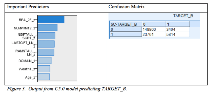
 From the above output it can be observed that there are 3,404 false positives and 23,761 false negatives. The error rate for this model is .149 and the model accuracy is .85. The probability of each donor for responding, also called the propensity score, is saved using the model and will be used later in the analysis. Although this tells us the best model based on error rate, this does not mean it is the most profitable model. For building the most profitable model to predict who to send a promotion to this analysis will be relooked at based on revenue. In the model maximizing profits, false negatives are worse than false positives because failing to contact a donor who would have responded positively to the promotion is losing much more money than the cost of mailing the promotion. False positives mean that the company only lost the cost of the mailing, $0.68, but ensured that they did not lose a potential responder. In the most profitable model this will be taken into account and to ensure as few false negatives as possible in order to maximize revenue.

 

PROBLEM 2. PREDICTING TARGET D

 

A model to predict TARGET_D is created. This is the amount that was donated. A regression model is used with the standardized variables and the categorical variables set as flag fields. The standard error, which is the square root of the mean square error, is used to estimate the error in the estimation/prediction of the model. The model with the least error, or smallest standard error, is seen as the most accurate. This number goes along with the adjusted r² value, which ranges from zero to one, where the lager the value the better the model performance. When building a regression model to predict TARGET_D, if the model is built on the original data set without being balanced the model produces adjusted r² values as low as 0.008. This is why it is important to make sure your training data set is balanced. Even with the training set balanced as discussed above with about 44% of TARGET_B=1, the model still produces poor results. To help the model improve some the balance node is adjusted to create an even higher percentage of donors. This method of overbalancing helps models perform better accuracy and in classification models also can account for some misclassification costs.

All variables are placed into the regression node and a stepwise method is used to model all possible combinations of variables in the regression. Using the output from this, the most significant variables are selected to be in the regression model predicting TARGET_D. Using only a regression model to predict TARGET_D the following figure 4 below lists the variables input into the model and the most significant of the predictors. This model produces an adjusted r² value of 0.150 and a standard error of estimates of 2.6778.

 

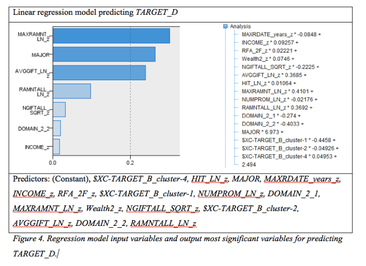
An estimated amount donated for each prospective donor is saved to the output for use in furthering to develop the predictive model. The model built tells us that the most significant predictor MAXRAMNT_LN_z. This can be due to the fact that the variable states the maximum amount of a gift to date. Those people that have donated large amounts at a time are more commonly to respond to a promotion. MAJOR is a significant predictor because as a flag variable it identifies those donors who are considered to be major donors or not. AVGGIFT_LN_z is also a significant predictor in the model because it tells us the average amount of gifts that that donor has given. This is obviously important in predicting how much someone will donate in the future by looking at what they have on average donated in the past.

 

PROBLEM 3. ESTIMATION MODEL

 

The propensity score obtained in problem 1 along with the donation estimates obtained in problem 2 combine to form expected donation. This is done by multiplying the two together for each donor. This is performed on the complete training data set of 181,779 donors and then also on the validation file. The validation file provided is a set of 10,000 records with the same variables as in the training file however without TARGET_B or TARGET_D. This file also has missing values, and dates that need changing. All data prep that was performed on the training file is performed on the validation file. This includes transforming and standardizing all variables in the same manor.

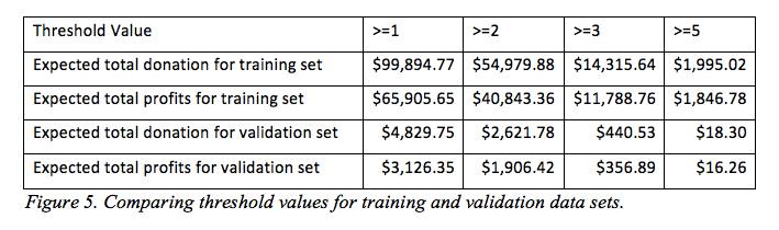
To determine which customers a promotion should be sent to, a threshold is chosen of an expected donation amount above which a letter will be sent to. The training and validation files are ran through the created model separately and the expected donation amount output is analyzed. Figure 5 shows the total expected donation and total expected profits for training and validation data sets for the multiple thresholds chosen. It is evident from the file that the lowest threshold of greater than or equal to one is the most profitable threshold is the most profitable for the company. For the training file this means a net revenue of $65,905.65. In order for this model to be obtained many different models were ran using different misclassifications, variables, and models to find the model with the highest expected total profits for the company. This best model found is used for the results seen here and the output file for the predictors.

The top ten prospected donors are listed in figure 6. These donors are based off of expected donation amounts. It is seen that within the top ten donors, only two of those are actually donors. Although this does not seem like many actual donors in our top predicted the two donors that are present donated far more than the average donor donation. This same table for the validation data set can be seen in figure 7 however in this case we do not know if the donors did in fact donate or not. All of the cases the prospected donors are predicted to donate.

 

CONTROLN	TARGET_B	TARGET_D	Propensity score	estimated donation	expected donation
185138	0	0	0.9375	15.41197	14.44872
144843	0	0	0.9375	15.35835	14.39845
14423	0	0	0.956522	14.93235	14.28312
185056	1	250	0.956522	14.78651	14.14362
14818	0	0	0.956522	14.69617	14.05721
14494	0	0	0.9375	14.82316	13.89671
14454	0	0	0.947368	14.46633	13.70494
14064	1	100	0.9375	14.41417	13.51329
14476	0	0	0.956522	13.98566	13.37759
5603	0	0	0.969697	13.75458	13.33777

Figure 6. Top ten prospects for training data set.

 

CONTROLN	TARGET_B Predicted	TARGET_D predicted	propensity score	expected donation
179802	1	8.531646	0.90625	7.731804
154040	1	6.259202	0.878788	5.500511
10095	1	5.209409	0.972973	5.068614
94363	1	6.068655	0.818182	4.965263
69540	1	5.36212	0.90625	4.859422
14528	1	5.952726	0.804124	4.786728
11873	1	5.861832	0.804124	4.713638
170894	1	5.164459	0.878788	4.538464
7706	1	5.014625	0.878788	4.406792
5371	1	5.007457	0.878788	4.400492

Figure 7. Top ten prospects for validation data set.

 

Net revenue generated is used as a predictor in how well your model performs and is calculated using the following equation:

“Sum (the actual donation amount – $0.68) over all records for
which you send a letter to the potential donor (i.e., TARGET_B = 1).”

The validation file includes 10,000 donors. If every donor was sent a promotion the average expected donation amount would be $0.793. This number is the average of all donations received in the training file. Sending a promotion to everyone would cost the company $0.68*10,000=$6,800. This means the net revenue for the null model would be $1,130. The goal of the model is to produce results to improve the profits of the null model. By the models and methods discussed above, those donors whom are predicted to make a donation amount above the expected donation threshold of 1 are selected to send a mailing to if the predicted TARGET_B predicts that they will donate. This was calculated using the equation “If Expected_Donation >= 1 then ‘$C-TARGET_B’ else 0 endif” in the derive node. Based on my model it is predicted that the net revenue will be $3,126.35. This is a 2.8% improvement from the null model. The predictions of those donors whom the promotion should be mailed to are indicated by a 1 in order to maximize profits.