Natalie Alexandra Sullo

 

Predicting Loan Defaults Analysis

Outline

A bank wants to review some of their loans to understand what causes borrowers to default. They’ve constructed a data set from loans issued over a five-year period. They want you to analyze the data and provide a brief report on which variables impact whether a loan is repaid.

Objectives

Analyze the provided data set to determine which variables impact whether a borrower pays in full (Loan Status = “Fully Paid”), or doesn’t (Loan Status = “Charged Off”). Please note any limitations or assumptions made of the data and in your analysis. How could your analysis be improved? What is missing from the data? If you use specific methodologies, please outline those in your response.

Data Source

The provided Loans Data Set.csv file contains all of the relevant data. The data set contains the following fields:

• Borrower ID: A unique identifier for the borrower.
• Loan Status: Whether the loan was paid in full or not.
• Amount Borrowed: The amount borrowed.
• Annual Income: The borrower’s annual income.
• State: The state where the borrower resides.
• Loan Term: The length of the loan.
• Interest Rate: The interest rate on the loan.
• Employment Duration: How long the borrower has been employed.
• Home Ownership: Whether the borrower is a homeowner.
• Verification: Whether the borrower’s income was verified.
• Issued: The date that the loan was issued.
• Earliest Credit: The date of the borrower’s earliest available credit.
• Purpose: What is the borrower planning to use the loan for?
• Delinquent Accounts (Past 2 Year): The borrower’s number of delinquent accounts from the past two years.
• Revolving Utilization Rate: The borrower’s revolving credit utilization.
• Number of Credit Lines: The borrower’s number of credit lines.

 

Exploratory Data Analysis

The following analysis was created using Excel and SPSS Modeler.

Within the Loans data set there are 39,786 unique records. The data is imported into SPSS Modeler and put through a data audit node to obtain an overview of the data as seen in Figure 1. This shows the field, a histogram of the data, the measurement or kind of data that the data is classified into, valid data points in each field, along with parameters of the data when applicable. All variables except for Revolving Utilization Rate have 39,786 data points. Revolving Utilization Rate has only 39,736 valid data points. There 50 missing data points are left blank. This will be looked into later in the analysis.

To ensure every Borrower ID number only appears once in the data (to make sure there is no repeated data) I used a distinct node to filter out any repeats, which showed that no data was filtered out so there were no repeats. I also ensured that there were no repeated data points with different Borrower ID numbers using the same distinct node to make sure there was no one line with identical data (when excluding Borrower ID). This showed there was no repeated data in the Loans data set.

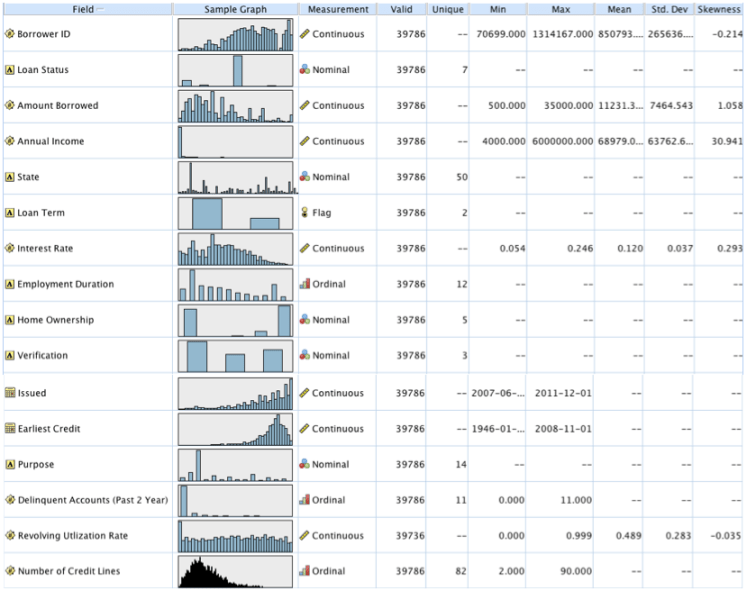Figure 1. Output from data audit node analyzing all variables.

Taking a closer look at the data I realized in order to utilize all of the variables, new variables were needed. I then went back to excel and created the following variables:

Issued_month: The month of the variable Issued.

Issued_Year: The year of the variable Issued.

Earliest Credit_Month: The month of the variable Earliest Credit.

Earliest Credit_Year: The year of the variable Earliest Credit.

DateDiff_Months_between_Earliest_credit_to_issued_date: The time in months between the Earliest Credit date and Issued date.

In excel I also changed Interest Rate and Revolving Utilization Rate into values, taking out the percentage, which was being read as a categorical variable in SPSS.

Importing this new data back into SPSS Modeler in place of the old data I then ran the data through a transform node to receive the output in Figure 2. This node takes the variables that are assumed continuous and creates histograms for each variable, along with the histograms for the variables with the inverse, logN, log10, exponential and square root transformations. This node makes it easy to pick which transformation makes the variables normally distributed. The transformation that is highlighted in yellow on each row is the chosen transformation that makes the variable most normally distributed. Some of the variables listed have no distribution chosen because there was no normal option or I believed that the variable would be better fit as a categorical variable such as Issued_month.

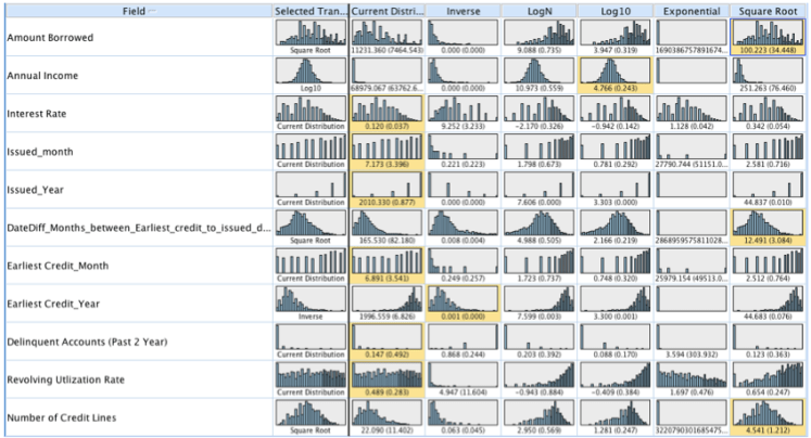Figure 2. Output from the Transform node.

After the transformation was chosen they were then created in SPSS Modeler using derive nodes. This was done with multiple variables using @FIELD as variables listed in the equations for the transformation. Square root, Log10 and the inverse were calculated using the equations ‘sqrt(@FIELD)’, ‘log(@FIELD+0.5)’ and ‘1/(@FIELD)’ respectively in the derive node. These new variables created were given the same variable name with the suffex ‘_Sqrt’, ‘_Log’, or ‘_Inverse’.

All continuous variables in the data set were then Z-score normalized; this includes the variables that were already transformed using sqrt, log or inverse transformations. This was done by first using the set globals node, which calculates mean, sum, min, max, stdev of all the variables to be used in the Z-score transformation. This transformation is also performed in the derive node using the equation ‘(@FIELD – @GLOBAL_MEAN(@FIELD)) / @GLOBAL_SDEV(@FIELD)’. Doing this converts all variables to the same scale with average of zero and standard deviation of one.

The partition node is then used to create a new field named Training=1 that separates the data into a training and a test set. The training set accounts for 75% of the data and is denoted with a 1. The test set accounts for 25% of the data and is denoted with a 2. This is done for potential future predictive analysis. The important thing to ensure when splitting is that there are equal proportions of each outcome of the target variable, Loan Status, in both the training and test sets. We examine the training and test sets below in figure 3a and figure 3b using a distribution graph with Loan Status overlay and also a matrix node to count each Loan Status option in each set to ensure equal proportions. Looking at the graph we can see that the distribution of loan status outcomes is similar in both the training (1) and test (2) sets and both have about 84% of their data as fully paid. This partitioning node can be set so that each time the stream is ran a new training and testing set will be chosen, different records will be chosen for different sets, and amounts will vary slightly. When I finally use this node for my analysis I end up taking out all other outcomes besides charged off and fully paid before I split this sent into training and test sets. This allows for a more accurate percent split and I later take out the other outcomes anyways.

Figure 3a. Example of a distribution graph of the training and test data sets with Loan Status overlay.

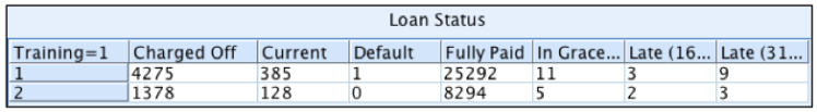Figure 3b. Example of the matrix node output which tells the count of the data in the training and test sets.

The next step in the data preparation process is to create two new variables using the reclassify node. These variables will make the model easier to build by making the outcomes in Loan Status number based. The first new variable created is Loan_Status_0_1_2, which takes Loan Status and transforms all ‘Fully Paid’ into 1 or a success, all ‘Charged Off’ into 0 or a failure, and all other options ie. ‘Current’, ‘In Grace Period’, ‘Late (31-120 days)’, ‘Late (16-30 days)’, and ‘Default’ into 2. These all other outcomes account for 547 data points, which is 1.37% of the data. This is done to make it easier to remove these ‘2’ options before modeling. This is the variable I end up using to create the model. The next variable created will be used to keep these other outcomes in for modeling.

The second variable created is named Loan_Status_0_1 that again transforms all ‘Fully Paid’ into 1 or a success, all ‘Charged Off’ into 0 or a failure, transforms ‘Current’ and ‘In Grace Period’ into 1 since they are not yet failures, and transforms ‘Late (31-120 days)’, ‘Late (16-30 days)’, and ‘Default’ into 0 or failures since they are leading towards failure. Both of these variables should be used as target variables in the predictive model and see which target produces more accurate results (only Loan_Status_0_1_2 is used in this analysis).

Missing Data Imputing

As I mentioned before there is 50 missing data points from Revolving Utilization Rate. There are a few different methods for dealing with missing data. If the missing data only affects a small number of the data set it is common to just eliminate those data points from the analysis. Doing this for this data set would probably have no great effect on the analysis since it is a small number of missing data. It is also common to replace the missing data with the mode of the variable. A third method is to use an appropriate analysis to model the variable and predict the missing data.

We use this third approach here by selecting the complete data of Revolving Utilization Rate_Z and building a linear regression model on the data. We choose the best model by building out the model with a stepwise function. This allows for multiple arrangements of the dependent variables put into the model and give output for all possible combinations. This helps determine which variables are significant to predict revolving utilization rate and then these variables are entered into the final regression model. Figure 4 shows the output of the most important variables in predicting Revolving Utilization Rate_Z. As you can see the variable with the greatest influence is Interest Rate_Z. This makes sense since the lower the credit card utilization the better a credit score, and generally the better the credit score the better the interest rate one can receive. Earliest credit year, number of credit lines, and delinquent accounts are the next three greatest predictors which also makes sense as all variables that would go into building credit affecting credit score and revolving utilization rate.

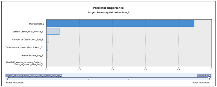Figure 4. Predictor importance output for a linear regression model estimating Revolving Utilization Rate_Z.

For an exact formula on how to calculate the predicted values, the output gives the formula: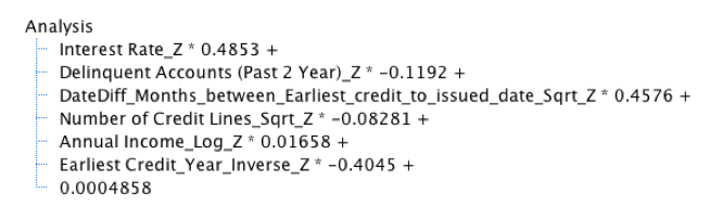The model also calculates these values for us and creates a brand new variable called $E-Revolving Utlization Rate_Z which is the predictions of the output model. We then replace the null values in our original data set with the predicted values for the 50 data points using the derive node and the equation “ if ‘Revolving Utlization Rate_Z’ = undef then round(‘$E-Revolving Utlization Rate_Z’) else ‘Revolving Utlization Rate_Z’ endif ”. This full equation is then used in the analysis for determining which variables impact whether a borrower pays in full or not.

Analysis

To determine which variables have the greatest impact on Loan Status we use a logistic regression to model the loan status outcome. This regression is used for data that have ordinal outcomes, such as a success or failure. Since the only desire is to know what variables impact whether a borrower pays in full (Loan Status = “Fully Paid”), or doesn’t (Loan Status = “Charged Off”) the other outcomes are removed from the analysis. This is done by using a select node and the command “ ‘Loan Status’ = ‘Fully Paid’ or ‘Loan Status’ = ‘Charged Off’ ”. This leaves my newly created variable Loan_Status_0_1_2 with only 0 and 1. This is the variable I will use from here on out to model loan status because it makes certain processes easier with 0 (failure) and 1 (success).

A logistic regression model is then built to predict Loan_Status_0_1_2 using the categorical variables and the normalized continuous variables. The output is analyzed and any non-significant variables are removed. The regression is redone until the most favorable model is selected. To determine this it is beneficial to examine the parameter estimations in the output. The ‘sig.’ value is looked at to make sure all the variables in the model are significant in determining the loan status outcome. It is also important to look at the Wald value in the same table because this value tells you by how much the variable affects the outcome. The higher this statistic the more the variable has an impact on the target variable (loan status). The -2 Log likelihood value is compared between models, and the lower this value the better because it explains more of the variance in the model. A sample of these values in the output can be seen in Figure 5. Figure 6 shows the most influential variables that affect loan status, which is also given in the output for a model.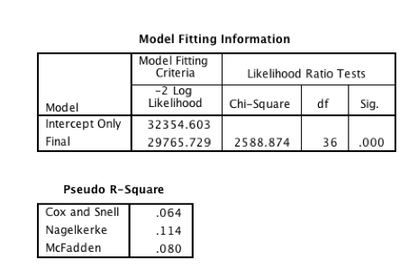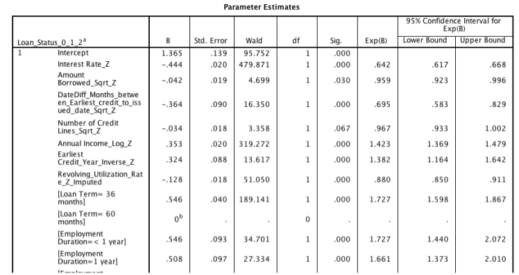Figure 5. Output of model fitting information and estimations from logistic regression model

Figure 6. Predictor Importance output from anlinear regression model predicting loan status.

To test out how the model works we will use the same variables to build a new model on the training data (Training=1). To do this, the training set is selected and another logistic regression is built from the training set using the same variables. This model is then put through the testing set (Training=2) to predict the loan status. Both this training and test set still only have loan status as fully paid, 1, or charged off, 0. All others were previously filtered out. The predictions can then be summarized in a table or exported out in a file. The predictions also come with a variable predicting how accurate the model believes the prediction is. This new data can then be compared with the real values to see how accurate the model is. Using this method many different variations of models can be tested to find the most accurate model. In this example the model predicts 8,507 of the 9,826 in the testing set correctly, or 86.8% accurately. This model can certainly improve with trying more variations and testing the accuracy.

There are many things that can be tested to improve upon this analysis. One of these mentioned before is to test both variables Loan_Status_0_1_2 and Loan_Status_0_1 as the target variable in the model without removing the “other” cases. This may not be necessary since these cases should eventually end in a success or a failure yet are incomplete so removing them could be more accurate, however trying different arrangements of models has the potential to improve the outcomes. Some variables may also perform better when they are binned together and may have a greater impact on predicting loan status then the variable did on its own. Also in the data it is visible that Interest Rate is not truly normal, and if taking this variable and splitting it up a model could be built on those members with lower interest rate and those with higher interest rate and the models can be combined after. This could allow for different models to be built on different kinds of members and allow for more accurate predictions.

Summary

When loans are created it is important for the lender to believe that the borrower will pay back the money in full. Knowing the greatest contributing variables for borrowers that pay versus borrowers that do not will help weed out failures. These major factors are the back bone of creating a predictive model to estimate if new borrowers coming in will pay back their loan and to what certainty we can guess that they will. Of all the models built it was common to see Interest Rate, Loan Term, Revolving Utilization Rate, and Purpose as the highest variables that impact whether a borrower pays in full or not.

Figure 7. View of stream in SPSS Modeler used to create analysis.